Example Application with Pool

When we first started parallelizing code, we used a short script that computed by by the Monte Carlo method.

Map requires an iterator for its second argument. We will manually divide the total number of “data throws” into chunks of roughly equal size on each process and store the result into a list myNumPoints. The Pool map method will then distribute the elements of the list, one to each cpu. This is called load balancing in parallel computing terms. Maximum efficiency generally occurs when each process performs approximately the same quantity of work. We also do not hard-code the number of processes, but will set an environment variable NUM_PROCS outside to select the core count.

"""
 This program estimates the value of PI by running a Monte Carlo simulation.

 NOTE:  This is not how one would normally want to calculate PI, but serves
 to illustrate the principle.
"""

import sys
import os
import math
import random
import numpy as np
import time
from multiprocessing import Pool
from functools import reduce

def pi(numPoints):
    """Throw a series of imaginary darts at an imaginary dartboard of unit
        radius and count how many land inside the circle."""

    numInside=0

    for i in range(numPoints):
        x=random.random()
        y=random.random()
        if (x**2+y**2<1):
            numInside+=1

    pi=4.0*numInside/numPoints
    return pi

def main():

    if (len(sys.argv)>1):
        try:
            numPoints=int(float((sys.argv[1])))
        except:
            print("Argument must be an integer.")
    else:
        print("USAGE:python MonteCarlo.py numPoints")
        exit()

    ncpus=int(os.getenv('NUM_PROCS'))
    print ('ncpus={}'.format(ncpus))
    chunks=numPoints%ncpus
    myNumPoints=[numPoints//ncpus+1]*chunks+[numPoints//ncpus]*(ncpus-chunks)
    print ('Points:', myNumPoints)

    pool = Pool(processes=ncpus)
    tic=time.time ()
    results = pool.map(pi,myNumPoints)
    ppi=reduce(lambda x,y:x+y,results)/ncpus
    print(ppi)
    toc=time.time ()
    pool.close(); pool.join()
    print("Parallel time on "+str(ncpus)+" cores:"+str(round(toc-tic,4)))

    #For comparison, run in serial
    tic=time.time()
    spi=pi(numPoints)
    print(spi)
    toc=time.time()
    print("Serial time:"+str(round(toc-tic,4)))

if __name__=="__main__":
    main()

Scaling

Most modern personal computers, including laptops, are multicore. If you are running on your own computer, test the code for a fairly small number of “dart throws.” You may change ncpus to a fixed integer corresponding to your computer’s core count. Start with 10000 and increase to 100000, then to 1000000. You may find that for a small number of throws, the serial time is faster than the multicore time. This is due to overhead, which includes the additional time required to set up the multiple processes and communicate between them. The result on one computer running Linux was

python mp_montecarlopi.py 10000
ncpus=4
Points: [2500, 2500, 2500, 2500]
3.1728
Parallel time on 4 cores:0.0011
3.1416
Serial time:0.001

 python mp_montecarlopi.py 100000
ncpus=4
Points: [25000, 25000, 25000, 25000]
3.1366
Parallel time on 4 cores:0.0055
3.13592
Serial time:0.0099

python mp_montecarlopi.py 1000000
ncpus=4
Points: [250000, 250000, 250000, 250000]
3.1393560000000003
Parallel time on 4 cores:0.0422
3.140852
Serial time:0.1007

python mp_montecarlopi.py 10000000
ncpus=4
Points: [2500000, 2500000, 2500000, 2500000]
3.1408840000000002
Parallel time on 4 cores:0.2585
3.1421124
Serial time:0.9626

As we might expect, the time for the serial run increases roughly linearly with the number of points. The parallel time seems to obey the same rule after the first test run; for larger runtimes the additional time to set up Multiprocessing becomes less significant. The value of $\pi$ also becomes more accurate as the number of “throws” increases.

We are increasing the amount of data per core without changing the number of cores. This is neither strong scaling nor weak scaling.

Exercise

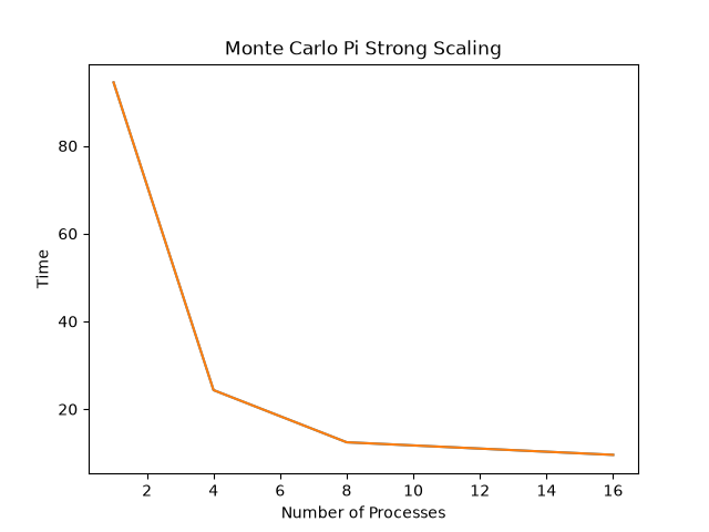
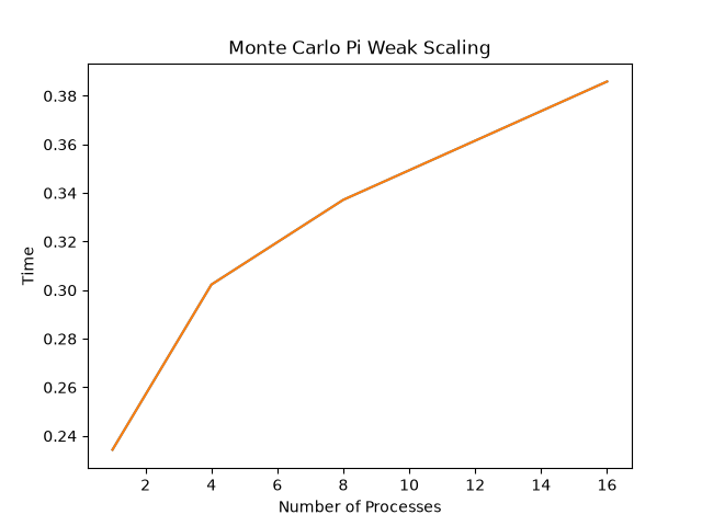
Run a strong scaling (same amount of work over a different number of cores) test and a weak scaling test (increase the amount of work but keep the amount per core the same). Plot the scaling results for the parallel timings.

Sample Results

Stong scaling

Weak scaling