Parallel Performance Analysis

Speedup and Efficiency

The purpose of making the effort to convert our programs to parallelism is a shorter time to solution. Thus we are interested in the speedup of a parallel code relative to running the same algorithm in serial. Speedup is a simple computation:

$$ Speedup = \frac{sequential\ execution\ time}{parallel\ execution\ time} $$

Let us consider a problem of size $n$, where $n$ represents a measure of the amount of work to be done. For example, it could be the first dimension of a square matrix to be inverted, or the number of pixels to analyze in an image. Now assume we will run this on $p$ processes. Let $$ \sigma (n) $$ be the part of the problem that is inherently sequential. Let $$ \phi (n) $$ be the part that is potentially parallelizable. Any parallelization will require some communication among the processes; the impact of this will be a function of both $n$ and $p$. Let us represent this as $$ \kappa (n,p) $$

On a single processor, the total time will depend on $$ \sigma (n) + \phi (n) $$ On $p$ processors, on the other hand, the time will depend on $$ \sigma (n) + \phi (n)/p + \kappa (n,p) $$ Therefore we can express the speedup as $$ \psi(n,p) = \frac{\sigma(n)+\phi(n)}{\sigma(n)+\phi(n)/p+\kappa(n,p)} $$

This simple formula shows that we would achieve the maximum possible speedup if $\sigma(n)$ and $\kappa(n,p)$ are negligible compared to $\phi(n)$. In that case we obtain the approximation $$ \psi(n,p)\approx \frac{\phi(n)}{\phi(n)/p} = p $$ Thus the ideal is that speedup should be linear in the number of processes. In some circumstances, the actual speedup for at least a limited number of processes can exceed this. This is called superlinear speedup. One fairly common cause of this is cache efficiency. When the problem is broken into smaller subdomains, more of the data may fit into cache. We have seen that cache is much faster than main memory, so considerable gains may be achieved with improved cache efficiency. Some other reasons include better performance of the algorithm over smaller data, or even moving to an algorithm that is better but only in parallel, since speedup is computed relative to the best sequential algorithm.

The efficiency is the ratio of the serial execution time to the parallel time multiplied by $p$, i.e. if $S$ is the speedup,

$$ \mathrm{Efficiency} = \frac{S}{p} $$

Using the above formal notation we obtain

$$ \epsilon(n,p)=\frac{\sigma(n) + \phi(n)}{p\sigma(n) + \phi(n) + p\kappa(n,p)}$$

From this it should be apparent that $$ 0 < \epsilon(n,p) \le 1 $$

Amdahl’s Law

Define $$ f = \frac{\sigma(n)}{\sigma(n)+\phi(n)} $$ This is the fraction of the work that must be done sequentially. Perfect parallelization is effectively impossible, so $f$ will never be zero.
In the speedup formula, consider the limiting case for which $\kappa(n,p) \to 0$. Thus $$ \psi(n,p) \lt \frac{\sigma(n) + \phi(n)}{\sigma(n) + \phi(n)/p} $$ Rewriting in terms of $f$ gives

$$ \psi \le \frac{1}{f + (1-f)/p} $$

In the case that $p \to \infty$ this becomes

$$ \psi \lt \frac{1}{f} $$

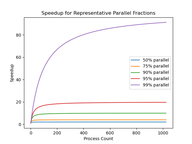
Thus the irreducibly sequential portion of the code limits the theoretical speedup. This is known as Amdahl’s Law.

Example

Suppose 95% of a program’s execution time occurs inside a loop that can be executed in parallel, and this is the only parallelizable part of the code. What is the maximum speedup we should expect from a parallel version of the program executing on 8 CPUs?  What is the efficiency? What is the maximum theoretical speedup?

In this case $$ f = 0.05 $$

So $$ \psi \le \frac{1}{0.05+0.95/8} = 5.92 $$ $$ \epsilon = \frac{t_{seq}}{8t_{seq}/5.92} = 0.74 $$ $$ \psi_{inf} = \frac{1}{.05} = 20 $$

Scalability

The Amdahl effect is the observation that as the problem size, represented by $n$, increases, the computation tends to dominate the communication and other overhead. This suggests that more work per process is better, up to various system limits such as memory available per core.

The degree to which efficiency is maintained as the number of processes increases is the scalability of the code. Amdahl’s Law demonstrates that a very high degree of parallelization is necessary in order for a code to scale to a large number of processes for a fixed amount of work, a phenomenon known as strong scaling.

Weak Scaling

Strong scaling over a large number of processors can be difficult to achieve. However, parallelization has other benefits. Dividing work among more cores can reduce the memory footprint per core to the point that a problem that could not be solved in serial can be solved.

• Strong scaling: the same quantity of work is divided among an increasing number of processes.

• Weak scaling: the amount of work per process is fixed, while the number of processes increases.

Amdahl’s law shows that strong scaling will always be limited. We must achieve a parallel fraction of close to 99% in order for the program to scale to more than around 100 processes. Many parallel programs are intended to solve large-scale problems, such as simulating atmospheric circulation or the dynamics of accretion disks around black holes, so will require hundreds or even thousands of processes to accomplish these goals; strong scaling is not feasible for these types of problem.

The counterpart to Amdahl’s Law for weak scaling is Gustafson’s Law. Here we fix not the size of the problem but the execution time. Using the same notation as before, with $f$ the fraction of the workload that must be executed sequentially, the sequential time that would be required for the problem size corresponding to $p$ processes will be $$ t_s = ft + (1-f)pt $$ where $t$ is the fixed execution time.
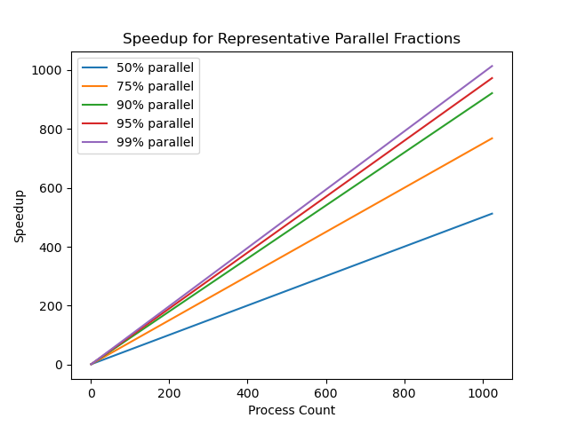
The speedup is $t_s/t$ which yields $$ \psi = f + (1-f)p $$ For weak scaling there is no upper limit on the speedup, and as $f \to 0$, $S \to p$. The ideal scaled speedup is thus linearly proportional to the number of processes.

The efficiency is $$ \epsilon = \frac{S}{p} = \frac{f}{p}+1-f $$ This expression ignores real-world complications such as communication and other system overhead, but it provides a guide for understanding weak scaling. In the case of $p \to \infty$, $\epsilon \to 1-f$. Therefore, as for Amdahl’s law, the sequential fraction will limit the speedup and efficiency possible. However, for weak scaling, lesser parallelization can still produce acceptable efficiencies.

Weak scaling allows a much larger workload to be run in the same time. A significant portion of scientific and engineering problems require a large to very large workload for problems of interest to be solved. For example, fluid dynamics is modeled better at higher numerical resolutions, but each computational cell adds to the problem size. Many problems, such as weather models, could not be solved at all at the resolution of interest without weak scaling.