The Heated Plate

Suppose we have a very flat rectangular metal plate. We immerse one edge in an ice bath at 0C and the other three edges in steam at 100C. The metal is a good conductor of heat. Heat loss from the surfaces will be ignored.

Intuitively we believe that heat will diffuse through the plate, but eventually a steady state will be reached. Mathematically, this is modeled by the heat diffusion equation, which is a time-dependent parabolic PDE. But with no change to the temperatures at the edges, eventually the transient flow of heat will settle into a steady state that depends on the temperature at the boundaries. We wish to predict the resulting temperature distribution.

We will skip to the equation that describes this steady state. It is the Laplace equation

$$ \nabla^{2}{u} = 0 $$

Writing out the Lapacian operator $\nabla^2$ in two dimensions, we have

$$ \frac{\partial^{2}{u}}{\partial{x}^{2}} + \frac{\partial^{2}{u}}{\partial{y}^{2}} = 0 $$

Here $u$ represents the temperature.

To solve this equation numerically, we will first discretize $x$, $y$, and $u$ onto a two-dimensional grid such as we used to study halo exchanges. Grids are typically represented by some type of array so we will denote the elements by indices $i$ and $j$. A point on the plate and its temperature will be represented in C++ as

x[i],y[i],u[i][j]

In Fortran as

x(i),y(i),u(i,j)

and in Python as

x[i],y[i],u[i,j]

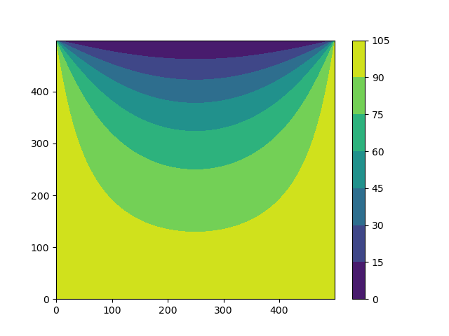
The Laplace equation is an elliptical PDE. The solution to elliptical PDEs is determined by the boundary conditions and the forcing function, if one is present (it is zero for the Laplace equation). We expect the solution to look something like this.