Profiling and Timing

The first step is usually to profile the code. Profiling can help us find a program’s bottlenecks by revealing where most of the time is spent. Keep in mind that most profilers work per function. If you do not have your code well separated into functions, the information will be less useful. Profilers are statistical in nature. They query the program to find out what it is doing at a snapshot during the run, then compile the results into a kind of frequency chart.

Python Profiler in the Spyder IDE

The Anaconda Spyder IDE provides an integrated Profiler that is easy to use. To profile your Python code follow these steps:

1. Open the Python script in the Editor pane. If your program is comprised of multiple files, open the script that contains the the main function.
2. In the Spyder menu, go to Run -> Profile.

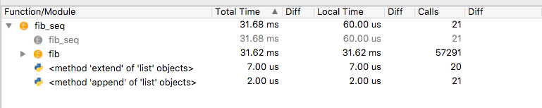
The results will be shown in the Profiler pane.

Exercise:

Open the fibonacci.py file and execute it with the Spyder Profiler. The code deliberately uses an inefficient algorithm. Let’s look at the output in the Profiler pane. What function was called most frequently and has the largest cumulative run time?

"""
Created on Mon Feb 3 17:56:40 2020

This program calculates the Fibonacci numbers for a range of integers.
The used algorithm is inefficient and chosen on purpose to demonstrate the
use of a Profiler.

@author: Karsten Siller
"""
def fib(n):
    # from http://en.literateprograms.org/Fibonacci_numbers_(Python)
    if n < 2:
        return n
    else:
        return fib(n-1) + fib(n-2)

def fib_seq(n):
    results = [ ]
    if n > 0:
        results.extend(fib_seq(n-1))
    results.append(fib(n))
    return results

if __name__ == '__main__':
    print (fib_seq(30))

A more detailed description of the Profiler option for Spyder can be found here.

Another popular IDE (integrated development environment) for Python is Pycharm by JetBrains. The profiler option is only available in the Professional (paid) version, but some UVA departments have a license for this version.

Profiling in Jupyter

To invoke the Python profiler in Jupyter, use the “magic” prun:

%prun code_line

for one line of code. To profile a code block use

%%prun
for i in range(10):
    a[i]=b[i]
    c[i]=a[i]**2

This runs the cProfile profiler. Prun will print a plain-text summary similar to the Profile window of Spyder.

Using the cProfile and pstats Modules in your script

Python includes the cProfile and profile packages. In Python 2, profile is a pure Python module with significant more overhead than the C extensions of cProfile (read the details). In Python 3, profile is cProfile by default. These packages can be used from the command line or in your Python scripts.

You can use the cProfile and pstats modules in your script to profile specific functions and save the profiling results to a file. Let’s assume that we have a module MyModule that defines a function myFunc to profile:

import MyModule
import cProfile
cProfile.runctx("MyModule.myFunc()", globals(), locals(), "Profile.result") 

Here globals() defines a set of global variables to be set for the profiling run. The locals() is a dictionary for arguments passed to the specific function to be profiled, i.e. MyModule.myFunc. The last argument, Profile.result, defines the file that the profiling output is written to.

The following code snippet can be used to implement profiling of the fib_seq function in the fibonacci.py script.

import cProfile,pstats

cProfile.runctx("fib_seq", globals(), {'n':30}, "Profile.result")
s = pstats.Stats("Profile.result") 
s.strip_dirs().sort_stats("time").print_stats()

Note the passing of {'n':30} to pass local arguments to the fib_seq function. The profiling stats are read from the Profile.result file, the path information of the involved Python modules is removed, and the output is sorted by time values before it is printed.

Other Tools

If you are running on your own system, you can install the snakeviz package. This enables you to view profiler output in a browser window. First you must generate the profile file. You can then invoke snakeviz from the command line with

snakeviz Profile.result

To use snakeviz from within an iPython shell or Jupyter notebook, first load it

load_ext snakeviz

Then use the “magics”

%snakeviz code_line

for a single line, or

%%snakeviz
a line
for i in stuff:
   more

for multiple lines.

Exercise:

Import the fibonnaci.py code to JupyterLab. Run prun. Try snakeviz if you wish to do so. Snakeviz requires Internet access while it is runnning; prun does not.

You can also install the line_profiler and memory_profiler tools.

conda install line_profiler
conda install memory_profiler

You can use pip if you are not working with Anaconda.

The line_profiler tool provides a special version of the Python interpreter, kernprof and defines a decorator @profile. To use it from the command line, add the decorator to any function you wish to profile.

@profile
def fib(n):
    # from http://en.literateprograms.org/Fibonacci_numbers_(Python)
    if n < 2:
        return n
    else:
        return fib(n-1) + fib(n-2)

@profile
def fib_seq(n):
    results = [ ]
    if n > 0:
        results.extend(fib_seq(n-1))
    results.append(fib(n))
    return results

You can then run on the command line

kernprof -l fibonacci.py

This produces a file script.py.lprof; in this specific case we now have

fibonacci.py.lprof

We must run it through the profiler to visualize it

python -m line_profiler script.py.lprof

Once installed, line_profiler can be invoked in Jupyter with the lprun magic:

%lprun -f fib fib_seq(30)

The functions to be profiled must be specified by the -f option to lprun.

Exercise

Run the line_profiler on the Fibonacci script.

Another potentially useful tool is the memory profiler. It is similar to line_profiler but for memory. To use memory_profiler rather than line_profiler, import from the module

from memory_profiler import profile

Now the @profile decorator will apply the memory profiler. Run with the -m option to Python

python -m memory_profiler fibonacci.py

This will print to the console, so be prepared to redirect the output.

In Jupyter the corresponding magics are memit and mprun. The memit magic will print the maximum memory usage, whereas mprun will generate the profile.

%load_ext memory_profiler
%memit fib_seq(30)

The mprun magic must work on modules imported from outside the notebook. We already have a fibonacci.py script so we can use that. However, we’ll need to change directory since Jupyterlab starts at the top-level folder.

import os
os.chdir("/home/myid/myfolder")
from fibonacci import fib
%mprun -f fib fib_seq(30)

We are using the fib_seq function that is in scope in Jupyter, but the fib function from the module.

Timing

Often we want to know exactly how long a particular code, or portion of the code, ran. Profiling adds some execution overhead and works only for functions; even line_profiler is function-based. For finer-grained data, we must measure the elapsed time directly.

The time module is available for longer segments of code.

import time
start_time=time.clock()
# do stuff
end_time=time.clock()
print ("Elapsed time is ",end_time-start_time)

Python 3 offers the timeit module for short snippets.

import timeit
print(timeit.timeit('"-".join(str(n) for n in range(100))', number=10000))

Since a single repetition of a command in Python may run too quickly to measure easily, we specify a number of repetitions (number=10000).

The Jupyter/iPython magics for timing are time and timeit.

%timeit fib_seq(10)
19.3 µs ± 108 ns per loop (mean ± std. dev. of 7 runs, 100000 loops each)

Timeit in Jupyter makes its own decision about how many repetitions to run. It also factors out system overhead. The time magic is like the Linux time command.

%time fib_seq(10)
CPU times: user 81 µs, sys: 5 µs, total: 86 µs
Wall time: 89.6 µs

With some tools in hand, we can now investigate how we can speed up our scripts.