Multiprocessing for Multicore Systems

Sometimes you cannot sufficiently speed up your program even with all optimization tricks. You may be able to take advantage of modern multicore processors to distribute the work across different cores. One popular programming model for multicore is threads. Threads are subprocesses launched by the initial process (the executable in most cases). Threads can be created and destroyed. Each thread should be assigned to its own core. Threads share a memory space and can also access the global memory of the system.

The Global Interpreter Lock (GIL)

Standard Python implements a GIL (global interpreter lock). Threads cannot be started within a single interpreter. A variety of workarounds to the GIL exist. For instance, Python 3 provides the threading module, which implements the Thread class. However, unless the programmer is familiar with low-level thread operations and is very careful, it is more likely to slow down the code than to speed it up.

The Process Class

In most cases, it is better to just start another Python process. The multiprocessing package handles this and manages communication among the processes. For the purpose of this tutorial we will experiment with a few different multiprocessing approaches. A detailed description can be found on the official Multiprocessing website.

One difference between true threads and a Multiprocessing process is that threads directly share memory and processes do not.

Import the package

from multiprocessing import Process

Define a function

def f(name): 
    print('hello from '+name)

if __name__ == '__main__': 
    ncpus=4
    for i in range(ncpus):
        p=Process(target=f,args=(str(i),)) 
        p.start()

The result may be something like

hello from 0
hello from 2
hello from 3
hello from 1

Notice that the responses are not in numerical order. In general, parallel programs do not guarantee ordering unless the library or the programmer forces it. In this case the processes results are printed as they arrive.

Note that multiprocessing requires a main() function and must be run inside it. This means that some examples, such as the multiprocessing.Pool examples, will not work in the interactive interpreter.

The Pool Class

For manager-worker problems, we can start a pool of workers. You can define a pool using an instance of the Pool class.

Pools work through data parallelization. The map method is analogous to the corresponding standard built-in “map” functional but distributes the data across the processes.

from multiprocessing import Pool 

def f(x): 
  return x*x 

if __name__ == '__main__': 
   pool = Pool(processes=4) 
   result = pool.map(f, range(1,11))
   
   # Print result
   print(result)  

   #Close out pool and have threads rejoin
   pool.close()
   pool.join()

In this example we created a Pool of four workers (Pool(processes=4)). The pool.map call submits a workload to the Pool of workers. The first parameter is the name of the function, in this case f, and the second argument defines the sequence of arguent(s) that need to be passed to the specified function f. Each element of the sequence is passed to f on one of the cores in use.

The map function is blocking; execution will not continue until the result is returned. Another version of map, map_async, is nonblocking. Execution continues while the computations are carried out. The communication is terminated when get is invoked.

from multiprocessing import Pool

def f(x):
  return x*x

if __name__ == '__main__':
   pool = Pool(processes=4)
   result = pool.map_async(f, range(1,11))

   #Do other things

   # Print result
   print(result.get())                      
   pool.close()
   pool.join()

The map method accommodates only one argument to the function. For Python 3.3 and later, starmap is available for multiple arguments. An efficient way to generate the required iterator of tuples is to use the zip() function.

from multiprocessing import Pool

def f(x,y,z):
   return x**y+z

if __name__ == '__main__':
   pool = Pool(processes=4)

   x=list(range(1,11))
   y=[2,1,3,4,2,3,1,0,3,2]
   z=list(range(50,61))
   fargs=zip(x,y,z)

   result = pool.starmap(f, fargs)

   # Print result
   print(result)
   pool.close()
   pool.join()

Another set of functions is apply and apply_async. The difference between the apply group and map/map_async is that apply returns the result from only one element of the pool. Like starmap, apply supports multiple arguments, but there is no starmap_async so if we need a nonblocking routine equivalent, we should use apply_async. We will need to collect the results ourselves.

from multiprocessing import Pool 

def f(x,y): 
  return x**y

if __name__ == '__main__': 
   pool = Pool(processes=4) 
   results=[]
   for x in range(1,11):
       results.append(pool.apply_async(f, (x,3)))
   allresults=[result.get() for result in results]
   # Print results
   print(allresults)  

Here is a more realistic example. Let’s parallelize our Monte Carlo pi solver (MonteCarloPiMC.py). Map requires an iterator for its second argument. We will manually divide the total number of “data throws” into chunks of roughly equal size on each process and store the result into a list myNumPoints. The Pool map method will then distribute the elements of the list, one to each cpu. This is called load balancing in parallel computing terms. Maximum efficiency generally occurs when each process performs approximately the same quantity of work. We also do not hard-code the number of processes, but will set an environment variable NUM_PROCS outside to select the core count.

"""
 This program estimates the value of PI by running a Monte Carlo simulation.

 NOTE:  This is not how one would normally want to calculate PI, but serves
 to illustrate the principle.
"""

import sys
import os
import math
import random
import numpy as np
import time
from multiprocessing import Pool
from functools import reduce

def pi(numPoints):
    """Throw a series of imaginary darts at an imaginary dartboard of unit
        radius and count how many land inside the circle."""

    numInside=0

    for i in range(numPoints):
        x=random.random()
        y=random.random()
        if (x**2+y**2<1):
            numInside+=1

    pi=4.0*numInside/numPoints
    return pi

def main():

    if (len(sys.argv)>1):
        try:
            numPoints=int(float((sys.argv[1])))
        except:
            print("Argument must be an integer.")
    else:
        print("USAGE:python MonteCarlo.py numPoints")
        exit()

    ncpus=int(os.getenv('NUM_PROCS'))
    print ('ncpus={}'.format(ncpus))
    chunks=numPoints%ncpus
    myNumPoints=[numPoints//ncpus+1]*chunks+[numPoints//ncpus]*(ncpus-chunks)
    print ('Points:', myNumPoints)

    pool = Pool(processes=ncpus)
    tic=time.time ()
    results = pool.map(pi,myNumPoints)
    ppi=reduce(lambda x,y:x+y,results)/ncpus
    print(ppi)
    toc=time.time ()
    pool.close(); pool.join()
    print("Parallel time on "+str(ncpus)+" cores:"+str(round(toc-tic,4)))

    #For comparison, run in serial
    tic=time.time()
    spi=pi(numPoints)
    print(spi)
    toc=time.time()
    print("Serial time:"+str(round(toc-tic,4)))

if __name__=="__main__":
    main()

Running on a Local Computer

Most modern personal computers, including laptops, are multicore. If you are running on your own computer, test the code for a fairly small number of “dart throws.” You may change ncpus to a fixed integer corresponding to your computer’s core count. Start with 10000 and increase to 100000, then to 1000000. You may find that for a small number of throws, the serial time is faster than the multicore time. This is due to overhead, which includes the additional time required to set up the multiple processes and communicate between them. The result on one computer running Linux was

$ python MonteCarloPiMC.py 10000
ncpus=4
Points: [2500, 2500, 2500, 2500]
3.0968
Parallel time on 4 cores:0.0068
3.13
Serial time:0.0056
$ python MonteCarloPiMC.py 100000
ncpus=4
Points: [25000, 25000, 25000, 25000]
3.14844
Parallel time on 4 cores:0.0245
3.1366
Serial time:0.0586
$ python MonteCarloPiMC.py 1000000
ncpus=4
Points: [250000, 250000, 250000, 250000]
3.1436
Parallel time on 4 cores:0.1963
3.14234
Serial time:0.5596

As we might expect, the time for the serial run increases roughly linearly with the number of points. The parallel time seems to obey the same rule after the first test run; for larger runtimes the additional time to set up Multiprocessing becomes less significant. The value of $\pi$ also becomes more accurate as the number of “throws” increases.

Running the Program on a Cluster

For those who have access to a high-performance computing cluster such as UVA’s Rivanna, Python scripts can be run in batch mode. Our example assumes the SLURM resource manager.

In order to execute our program on designated compute node(s), we need to write a simple bash script that defines the compute resources we need. We call this our job script. For our example, the job script pimc.sh looks like this:

#!/bin/bash
#SBATCH -N 1
#SBATCH --cpus-per-task=4
#SBATCH --account=your_allocation
#SBATCH -p instructional
#SBATCH -t 10:00:00

echo Running on `hostname`

module purge
module load anaconda/5.2.0-py3.6

# set the NUM_PROCS env variable for the Python script
export NUM_PROCS=${SLURM_CPUS_PER_TASK}
python MonteCarloPiMC.py 100000000

You can view this script in a text editor on Rivanna. If you are connected through a FastX Mate session, go to the menu Applications -> Accessories –> Pluma Text Editor.

The #SBATCH directives define the compute resources (-N, --cpus-per-task, -p), compute wall time (-t), and the allocation (-A) to be used. -N 1 specifies that the job runs on a single node. With --cpus-per-task we request the number of cpu cores for the job. By increasing the number for --cpus-per-task we can take advantage of multiple cpu cores and set up a bigger pool of workers. Ideally we want to match the worker pool size with the number of cpu cores.

Submitting the job

The job must be submitted to the job scheduler with a specific command. On Rivanna we use the Simple Linux Utility Resource Manager (SLURM) and the sbatch command for job submission.

Open a terminal window and execute this command:

sbatch pimc.sh

After submission you should see output like this:

Submitted batch job 9024339

The integer number resembles a unique job id.

Checking the Job Status

You can check the status of your jobs by running either one of these commands:

• squeue -u YOUR_ID
• sacct

The squeue command show all active jobs, either pending or running. The sacct command shows the history of your jobs whether they are pending, running, completed, cancelled or failed.

You can find more details about SLURM and job management on our website.

Checking the Output File

SLURM creates output files for each job that log the information that the program prints to stdout and stderror during the job run. The file(s) will also include information in case the job run was aborted. By default the name of the SLURM output file is slurm-<JOB_ID>.out. Check the directory in which you executed the sbatch command for a SLRURM output file and open it in a text editor.

Exercises: Rerun the job using 2, 4, or 8 cpu cores. In order to do this, open the pimc.sh, change the --cpus-per-task option accordingly, save the file, and resubmit the job script from the terminal window with the sbatch command.

Scaling

When we run the exercise with 10^9 points we may obtain results like these (on one particular workstation):

CPU cores	Run time	Scaling
1 (serial)	402 sec	1
4	109.5 sec	3.67
8	60.5 sec	6.64
16	32.5 sec	12.37

If we plot time versus number of cores we obtain the following graph. The orange line is ideal scaling, where the total time is the serial time divided by the number of cores used. The blue line shows the actual runtime and speedup achieved.

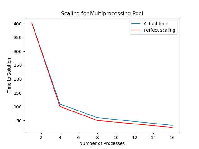
Our actual scaling in this case is quite close to perfect. This has a lot to do with our problem; the amount of time taken is mostly proportional to the number of throws to be calculated. Not all problems scale this well.

Combining Approaches

If we are using Anaconda we can use Numba and Multiprocessing together. On the same workstation this reduced the serial time to 12.8 seconds and the time on 4 cores to 5.8 seconds. The poorer scaling here could be due to the time required being so small that the overhead became dominant.

Further Information

The official documentation for Multiprocessing is here.

This tutorial has some examples for using the Process class.

A good tutorial for both Processing and Pool is here. It also introduces the Queue, which we have not discussed.