Distributed Parallel Programming

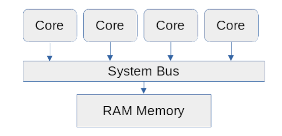
Nearly all recent computers, including personal laptops, are multicore systems. The central-processing units (CPUs) of these machines are divided into multiple processor cores. These cores share the main memory (RAM) of the computer and may share at least some of the faster memory (cache). This type of system is called a shared-memory processing or symmetric multiprocessing (SMP) computer.

Schematic of an SMP system

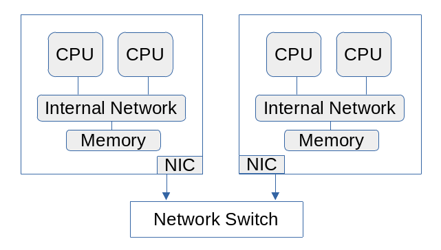
A computing cluster consists of a group of computers connected by a network. High-performance clusters nearly always have a network that is faster than the Ethernet used by consumer devices. Many use a network called InfiniBand. A cluster is thus a distributed-memory processor (DMP). Each computer, usually called a node, is independent of the others and can exchange data only through the network.

Multiprocessing works only on a single computer with multiple computing cores (SMP). If you have access to a computing cluster you can use distributed parallelization to run your program on multiple computers (DMP) as well as multiple cores per computer. This requires a communications library.

Schematic of a DMP system

Before considering parallelizing your program, it is highly desirable to spend some time optimizing the serial version. Particularly if you can utilize NumPy and Pandas effectively, you may not need to try to parallelize the code. If you still need to do so, a well-optimized, clearly-written script will make the work much easier.

Dask

Dask is a framework for distributed applications. It works with NumPy, Pandas, and Scikit-Learn, as well as some less common packages that have been customized to utilize it. It is primarily used to distribute large datasets.

Dask breaks the work into tasks and distributes those tasks. It can use multicore systems easily. With some care, it can also use multiple nodes on a cluster if that is available. A task may be reading a file, or doing some work on a portion of a large dataframe, or processing JSON files. To accomplish this, Dask constructs a task graph. This lays out the order in which tasks must occur. Independent tasks can be run in parallel, which can considerably speed up the time to solution. Dask is lazy and results are collected only as needed.

Our examples are taken from the Dask documentation. We cover only the basics here; a more complete tutorial can be downloaded as Jupyter notebooks.

Dask is best utilized for problems for which the dataset does not fit in memory. Some overhead is associated with it, so if your optimized NumPy or Pandas code can handle the problem, it is better to use those standard packages.

Dask Arrays

Dask arrays are much like NumPy arrays, but are decomposed into subunits that Dask generally calls chunks. In the language of parallel computing, we call this data decomposition.

>>>import dask.array as da
>>>x = da.random.random((10000, 10000), chunks=(1000, 1000))

Here we have created a two-dimensional array and broken it into 100 1000x1000 subarrays. The full-sized array is not actually created so we do not need the memory required for it. This is a general rule; avoid creating large global arrays. Large, memory-hungry arrays can be slow to process or, if they do not fit in any available memory, can make the problem impossible to solve on most computers.

Most, but not all, NumPy functions and methods are available for Dask arrays.

>>>x.mean()

This returns

dask.array<mean_agg-aggregate, shape=(), dtype=float64, chunksize=(), chunktype=numpy.ndarray>

This is because the Dask functions set up a computation but most do not execute it until told to do so. To get our answer we must invoke the compute method.

>>>x.mean().compute()
0.5000237776672359

Certain operations that require the full result, such as plotting, will automatically invoke compute but it can always be done explicitly.

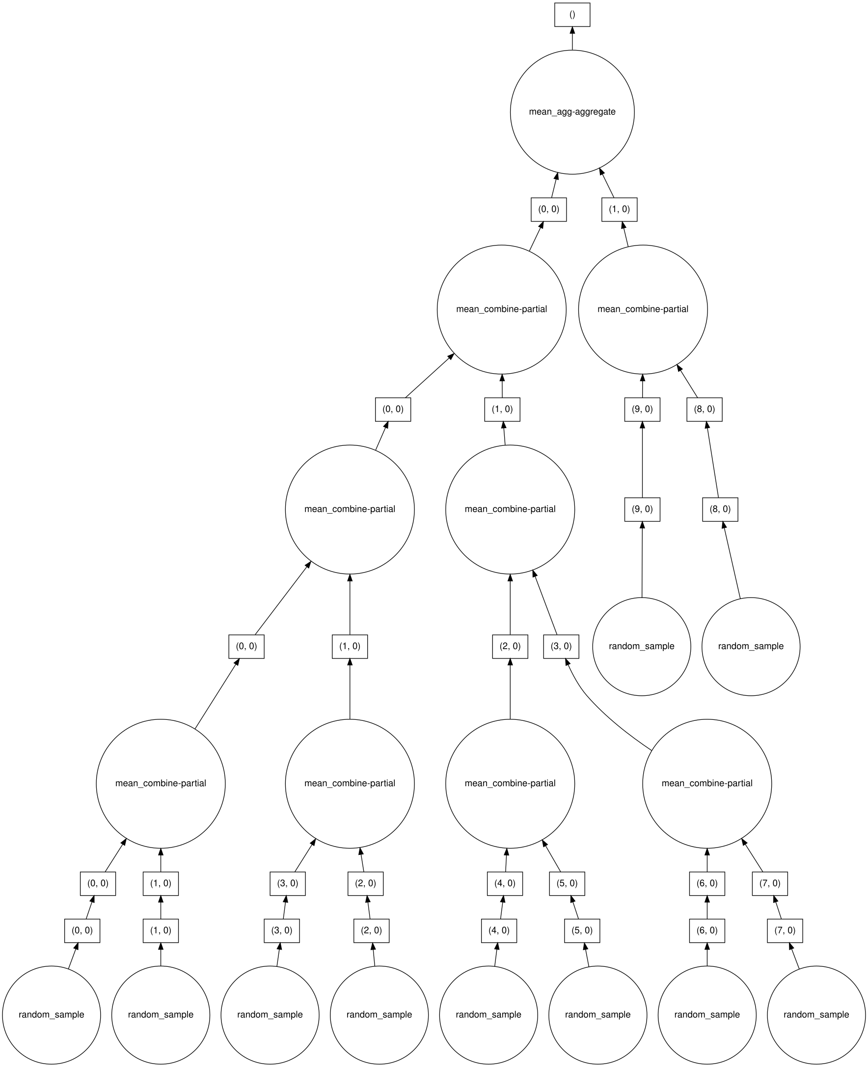
To visualize the task graph for a given Dask object, be sure that graphviz is installed (python-graphviz for conda). The visualize method for a Dask object will then produce the graph. If run at the command line, the result should be written to a file. Within a Jupyter notebook, the image will be embedded.

Example

import dask
import dask.array as da

x = da.random.random((100, 100), chunks=(10, 100))
y=x.mean()
# visualize the low level Dask graph after optimizations
y.visualize(filename="da_mean.svg", optimize_graph=True)

Expected result

Dask Dataframes

Dask also has an infrastructure built atop Pandas. As for NumPy, many but not all Pandas functions and methods are implemented.

>>>import dask
>>>import dask.dataframe as dd
>>>df = dask.datasets.timeseries()
>>>df

This is also lazy:

Dask DataFrame Structure:
                   id    name        x        y
npartitions=30
2000-01-01      int64  object  float64  float64
2000-01-02        ...     ...      ...      ...
...               ...     ...      ...      ...
2000-01-30        ...     ...      ...      ...
2000-01-31        ...     ...      ...      ...
Dask Name: make-timeseries, 30 tasks

Only the structure of the dataframe has been established.

We can invoke Pandas functions, but as for arrays we must finalize the results.

>>>df2 = df[df.y > 0]
>>>df3 = df2.groupby('name').x.std()
>>>df3.compute()

Exercise In a Jupyter notebook or Spyder interpreter, run the Dataframe examples above. Now run

>>>import matplotlib.pyplot as plt

or in Jupyter

%matplotlib inline

Then

>>>df[['x', 'y']].resample('1h').mean().head()
>>>df[['x', 'y']].resample('24h').mean().compute().plot()

Run

>>>plt.show()

if necessary.

The Dask version of read_csv can read multiple files using wildcards or globs.

>>>df = dd.read_csv('myfiles.*.csv')

When creating a Dataframe, Dask does attempt to assign a type to each column. If it is reading multiple files it will use the first one to make this determination, which can sometimes result in errors. We can use dtype to tell it what types to use.

>>>df = dd.read_csv('myfiles.*.csv',dtype={'Value':'float64'})

Example

import numpy as np
import pandas as pd
import dask
import dask.dataframe as dd

df = dask.datasets.timeseries('2000','2010',freq='2H')
print(df.head())

df2 = df[df.y > 0]
df3 = df2.groupby("name").x.std()
print(df3)
print(df3.compute())
df4=df.groupby("name").aggregate({"x": "sum", "y": "max"})
print(df4.compute())

Dask Delayed

Another example of lazy evaluation by Dask is delayed evaluation. Sometimes functions are independent and could be evaluated in parallel, but the algorithm cannot be cast into an array or dataframe. We can wrap functions in delayed, which causes Dask to construct a task graph. As before, results must be requested before actual computations are carried out.

Example

import dask
from dask.distributed import Client, progress
import time
import random

def inc(x):
    time.sleep(random.random())
    return x + 1

def dec(x):
    time.sleep(random.random())
    return x - 1

def add(x, y):
    time.sleep(random.random())
    return x + y

if __name__=="__main__":
   client = Client(threads_per_worker=4, n_workers=1)

   zs=[]
   for i in range(20):
       x = dask.delayed(inc(i))
       y = dask.delayed(dec(x))
       z = dask.delayed(add(x, y))
       z=z.compute()
       zs.append(z)
   print(zs)

   client.close()


It is also possible to invoke delayed through a decorator.

@dask.delayed
def inc(x):
    time.sleep(random.random())
    return x + 1

@dask.delayed
def dec(x):
    time.sleep(random.random())
    return x - 1

@dask.delayed
def add(x, y):
    time.sleep(random.random())
    return x + y

Dask Bags

Dask Bags implement collective operations like mapping, filtering, and aggregation on data that is less structured than an array or a dataframe.

Example

Download the data. Unzip it where the Python interpreter can find it. If using Jupyter make sure to set the working folder and then provide the path to the data folder.

import dask.bag as db
b = db.read_text('data/*.json').map(json.loads)
b
b.take(2)  # shows the first two entries
c=b.filter(lambda record: record['age'] > 30)
c.take(2)
b.count().compute()

Exercise Run the above example. Why does the expression b not show any values?

Xarray

Xarray is a project that extends Pandas dataframes to more than two dimensions. It is able to use Dask invisibly to the user, with some additional keywords.

>>>import xarray as xr
>>>ds = xr.tutorial.open_dataset('air_temperature',
                              chunks={'lat': 25, 'lon': 25, 'time': -1})
>>>da = ds['air']
>>>da

The result shows the chunks layout but not the actual data. Without the chunks argument when the dataset was initiated, we would have an ordinary Xarray dataset.

Xarray is particularly well suited to geophysical data in the form of NetCDF files, but can also handle HDF5 and text data.

Dask and Machine Learning

Machine learning is beyond our scope here, but we will make a few comments. Dask can integrate with scikit-learn in the form of Dask-ML.

>>>import numpy as np
>>>import dask.array as da
>>>from sklearn.datasets import make_classification
>>>X_train, y_train = make_classification(
       n_features=2, n_redundant=0, n_informative=2,
       random_state=1, n_clusters_per_class=1, n_samples=1000)
>>>X_train[:5]
>>>N = 100
>>>X_large = da.concatenate([da.from_array(X_train, chunks=X_train.shape)
                             for _ in range(N)])
>>>y_large = da.concatenate([da.from_array(y_train, chunks=y_train.shape)
                             for _ in range(N)])
>>>X_large
>>>from sklearn.linear_model import LogisticRegressionCV
>>>from dask_ml.wrappers import ParallelPostFit
>>>clf = ParallelPostFit(LogisticRegressionCV(cv=3), scoring="r2")
>>>clf.fit(X_train, y_train)
>>>y_pred = clf.predict(X_large)
>>>y_pred
>>>clf.score(X_large, y_large)

Dask can also be used with Pytorch. See the documentation for an example.

MPI

The most widely used general-purpose communications library for distributed parallelization is MPI, the Message Passing Interface.

MPI works on multicore systems as well as multinode, but the programming model is still different from threads.

In MPI each process has an ID called its rank. Ranks are numbered from 0 to n-1, for n processes. Each process runs completely independently. No process shares memory with any other process whether running on the same node or not. All communications occur over the network. To use MPI the programmer must manage the distribution of the data to different processes and the communication among the processes.

MPI messages are identified by an “envelope” of metadata. This consists of the destination, the source (the “return address”), a communicator (a group of processes that will be exchanging information), and optionally a tag. A communicator consisting of all processes, called COMM_WORLD, is set up when the MPI program is initiated.

The process with rank 0 is usually called the root process. Since the mimumum number of processes is 1, the root process is the only one that is guaranteed to be present. For this reason it is usually used to manage various bookkeeping tasks as well as input/output.

The mpi4py Package

The most popular direct way to use MPI with Python is the mpi4py package. It is not included in the base Anaconda distribution. To install it into your environment in an HPC cluster such as Rivanna, load the appropriate modules for compiler and an MPI distribution. It is important that a command mpicc provided by your HPC site be first in your path, since that should have been set up to communicate properly with your resource manager (SLURM etc.)

module load gcc/9.2.0
module load openmpi
module load anaconda
pip install --user mpi4py

You must use pip rather than conda because conda will install precompiled binaries and you must compile mpi4py explicitly.

MPI consists of dozens of functions, though most programmers need only a fraction of the total. The mpi4py package has implemented most of them using a “Pythonic” syntax, rather than the more C-like syntax used by other languages. One peculiarity of mpi4py is that only particular types may be communicated; in particular, only NumPy NDArrays or pickled objects are supported. To simplify our discussion, we will ignore the versions for pickled objects. The requirement that NumPy arrays be sent means that even single values must be represented as one-element NumPy arrays.

MPI requires more advanced programming skills so we will just show an example here. Our Monte Carlo pi program is well suited to MPI so we can use that.

"""
 This program estimates the value of PI by running a Monte Carlo simulation.
 Imagining a virtual dart board of radius 1 (centered at the origin) and
 inscribed within a square of side-length 2 (centered at the origin), the
 program throws a large number of "darts" at the board and counts how many
 of the darts land within the circle.  Because we know that a circle of
 radius 1 has an area of PI, and because we know that a square of side-length
 2 has an area of 4, we can approximate the value of PI by considering that
 the ratio of the number of darts inside the circle to the number of darts
 outside the circle but in the square should be equal to the raio of PI over
 4.  Simplified, PI = 4 ! (dartsInside / dartsTotal).

 NOTE:  This is not how one would normally want to calculate PI, but serves
 to illustrate the principle.
"""

import sys
import os
import math
import random
import numpy as np
import time
from mpi4py import MPI

def pi(numPoints):
    """Throw a series of imaginary darts at an imaginary dartboard of unit 
        radius and count how many land inside the circle."""

    numInside=0
  
    for i in range(numPoints):
        x=random.random()
        y=random.random()
        if (x**2+y**2<1):
            numInside+=1

    pi=4.0*numInside/numPoints
    return pi

def main():

    if (len(sys.argv)>1):
        try:
            numPoints=int(float((sys.argv[1])))
        except:
            print("Argument must be an integer.")
    else:
        print("USAGE:python MonteCarlo.py numPoints")
        exit()

    myrank = MPI.COMM_WORLD.Get_rank()
    nprocs = MPI.COMM_WORLD.Get_size()

    chunks=numPoints%nprocs
    myNumPoints=[numPoints//nprocs+1]*chunks+[numPoints//nprocs]*(nprocs-chunks)

    tic=time.time ()
    mypi=np.ones(1)*pi(myNumPoints[myrank])
    ppi=np.zeros(1)
    MPI.COMM_WORLD.Reduce(mypi, ppi, op=MPI.SUM, root=0)
    ppi/=float(nprocs)
    toc=time.time()
    if myrank==0:
        print("Pi is approximately",ppi[0])
        print("Parallel time on "+str(nprocs)+" cores:"+str(round(toc-tic,4)))

        tic=time.time()
        spi=pi(numPoints)
        print("Pi is approximately ",spi)
        toc=time.time()
        print("Serial time:"+str(round(toc-tic,4)))

if __name__=="__main__":
    main()

The first invocation of MPI is the call to Get_rank. This returns the rank of the process that calls it. Remember that each MPI process runs as a separate executable; the only way their behaviors can be controlled individually is through the rank. This call also initializes MPI; a separate MPI.Init is not required. The next line allows us to find out how many processes are in COMM_WORLD. The number of processes for MPI programs is always set outside the program, and should never be hardcoded into the source code.

Next we divide up the number of “throws” into roughly equal chunks, just as we did in the corresponding Multiprocessing example. The same list is generated, but we use myrank to select the element of the list that each rank will use.

After this each process invokes the pi routine using myNumPoints for its rank. We need to collect all the estimates and average them. The reduction collects the results from each rank (in rank order) and applies the “op” (operation). A reduction must be a binary operation that returns another object of the same type; the operation is applied along the sequence. In this case we want the sum so we add the result from rank 0 to that from rank 1, then we take that sum and add the result from rank 2, and so forth. Dividing by the number of processes provides the average.

The Reduce function returns each result to the process regarded as the root, which would normally be 0 as it is in this case, and root carries out the operation. Thus only the root process knows the final result. We then select root to print out the value.

This example reruns the problem without distributing the throws in order to obtain a serial time for comparison purposes. Of course, a real application would not do that.

Running the MPI Python Program on Rivanna

In order to launch multiple tasks (or processes) of our program, we run this program through the MPI executor. On our HPC cluster this is srun.

srun python MonteCarloPiMPI.py 1000000000

Note: you cannot launch the MPI program with srun on the Rivanna login nodes. In order to execute our program on designated compute node(s), we need to write a simple bash script that defines the compute resources we need. We call this our job script. For our example, the job script pimpi.sh looks like this:

#!/bin/bash
#SBATCH -N 1
#SBATCH --ntasks-per-node=8
#SBATCH --account=your_allocation
#SBATCH -p instructional
#SBATCH -t 10:00:00

echo Running on `hostname`

module purge

#Load the versions of gcc, MPI, and Python/Anaconda in which you installed mpi4py
module load gcc
module load openmpi
module load anaconda

srun python MonteCarloPiMPI.py 100000000

The #SBATCH directives define the compute resources (-N, --ntasks-per-node, -p), compute wall time (-t), and the allocation account (--account) to be used. -N 1 specifies that all MPI tasks should run on a single node. We are limiting the number of nodes for this workshop so that everyone gets a chance to run their code on the shared resources.

Submitting the job:

Open a terminal window and execute this command:

sbatch pimpi.sh

Checking the job status:

Check the job status with the squeue -u or sacct commands as described in the Multiprocessing section.

Checking the output file:

Open the slurm-XXXXXX.out files in a text editor and record the total run time for the job.

Exercise

Rerun the MPI job using 1 or 4 cpu cores by changing the --ntasks-per-node option.

Scaling

On the cluster, the timings are very similar to Multiprocessing on the workstation.

CPU Cores Run Time
1 (serial) 400 sec
4 102 sec
8 60 sec
16 31 sec

Dask-MPI

Dask can use mpi4py on a high-performance cluster. First install mpi4py according to the instructions in the previous section, then pip install --user dask-mpi.

Schedulers

We have not discussed Dask schedulers previously. The scheduler is a process that managers the workers that carry out the tasks. We have been implicitly using the single-machine scheduler, which is the default. Within the single-machine scheduler are two options, threaded and processes. The threaded single-machine scheduler is the default for Dask Arrays, Dask Dataframes, and Dask Delayed. However, as we discussed with Multiprocessing, the GIL (Global Interpreter Lock) inhibits threading in general. Most of NumPy and Pandas release the GIL so threading works well with them. If you cannot use NumPy and Pandas then the processes scheduler is preferred. It is much like Multiprocessing.

To use Dask-MPI we must introduce the Dask distributed scheduler. The distributed scheduler may be preferable to processes even on a single machine, and it is required for use across multiple nodes.

Running Dask-MPI

We will discuss here only the batch interface for Dask MPI. Dask-MPI provides an initialize function that initializes MPI and sets up communications. You must then start a Client cluster to connect the workers. Dask-MPI uses rank 0 for the manager process and rank 1 to mediate between manager and workers, so you must request at least 3 processes. Close the cluster at the end of your script to avoid error messages about terminated processes.

Example Convert the “timeseries” example to Dask MPI.

import os
import dask
import dask_mpi as dm
import dask.distributed as dd
import dask.dataframe as ddf
from dask.distributed import Client

# Initialize Dask cluster and store worker files in current work directory
dm.initialize(local_directory=os.getcwd())

#Connect clients
client = Client()

df=dask.datasets.timeseries()
df2=df[df.y>0]
df3=df2.groupby('name').x.std()
df3.compute()
print("Finished")
client.close()

Run this simple example with

#!/bin/bash
#SBATCH --ntasks=4
#SBATCH -p standard
#SBATCH -A hpc_build
#SBATCH -t 00:10:00

module load gcc/9.2.0
module load openmpi
module load anaconda

export OMPI_MCA_mpi_warn_on_fork=0
srun python dask_df_mpi.py

The OMPI_MCA environment variable suppresses a warning message that is seldom relevant.

Using Dask-MPI is not difficult, especially in batch mode, but users interested in trying it should be sure to first understand the distributed scheduler, then study the online examples carefully. Dask-MPI does not require explicit calls to MPI but with the convenience comes some loss of control; the algorithm must be suited to the distributed scheduler. More information may be found in the documentation.

Full documentation for Dask-MPI is here.

Previous
Next