Data

Fiji Installation

Fiji is available on Windows, Mac, and Linux platforms and can be downloaded directly from the Fiji website: https://fiji.sc/. Fiji is a portable application, meaning it doesn’t require an installer. To use Fiji, simply download and unzip the application, and then you are able to start it.

• MacOS X: The Fiji application should be installed in the user’s home directory rather than the default Applications folder.
• Windows 7 & 10: The Fiji application should be installed in the user’s home directory rather than the default C:\Program Files directory.
• Linux: The Fiji application should be installed in a directory where the user has read, execution, and write permissions, e.g. the user’s home directory.

Introduction

Image Processing & Analysis

• Image Filtering (removal of noise and artifacts)
• Image Enhancement (highlight features of interest)
• Image Segmentation (object recognition)
• Quantitative Image Feature Description (object measurements)

Image Processing Applications

• Photography & cinematography
• Digitization of non-digital documents -> text mining
• Natural sciences, engineering
• Forensics, e.g. finger print matching
• Quality control, e.g. in semiconductor fabrication
• Satellite surveillance, e.g. weather forecasting, terrain usage analysis
• Autonomously operating machinery (cars, etc.)
• Automatic cataloging of pictures on the web

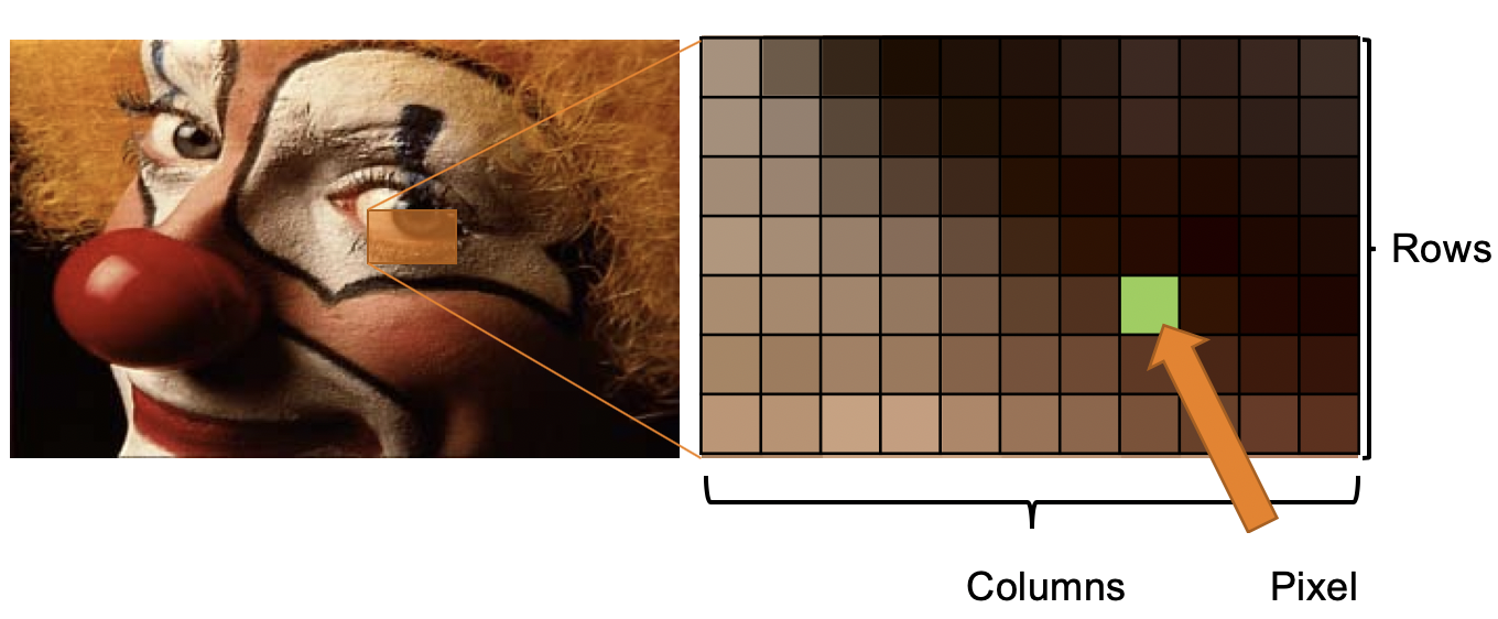
The Digital Representation of an Image

• 2D images are 2D arrays of numbers organized in rows and columns
• The intersection of row and column is a pixel
• Each pixel is represented as an intensity value (e.g. between 0-255)

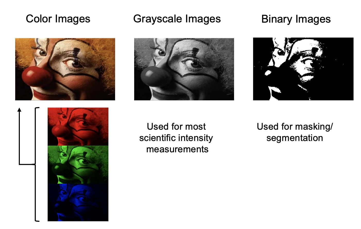
Fiji can handle image files in various file formats and pixel encodings, e.g. color images (RGB, HSB, etc.), grayscale images, and binary images.

Color images use 8-bit encoding for each channel (e.g. RGB: 256 intensity values for red, green, and blue).

Pixels in grayscale images may be encoded as 8-bit integer (256 intensity levels), 16-bit integer (65536 intensity levels), or 32-bit float (decimal number) values.

Binary images are a special type of 8-bit grayscale images that only contain the pixel values 0 (black) or 255 (white). They are used for masking and segmentation of object areas of interest in an image.

Image Processing & Analysis

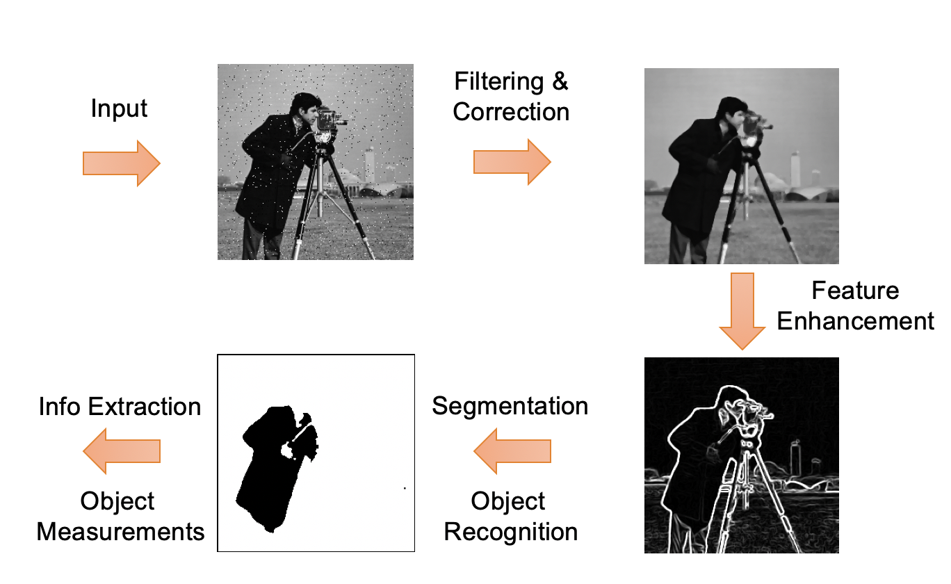
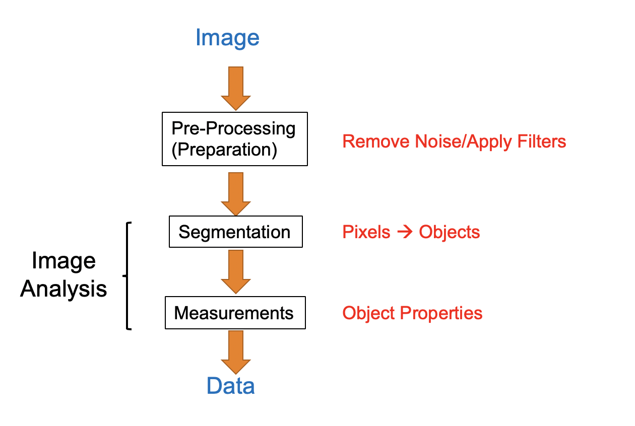
Image processing and analysis procedures often share a common workflow as shown here.

The original image (or raw data) that serves as input for the image processing pipeline may contain background noise that may need to be removed by applying specifc image filters.

The cleaned-up image may then be processed to enhance certain features, e.g. highlight object edges.

The enhanced image can then be converted into binary image masks that define groups of pixels as objects. Based on these masks, objects of interest can be classified and analyzed for size, geometry, pixel intensities, etc..

Basic Operations in ImageJ/Fiji

• Handling Image Files
• Working with Image Channels
• Image Montage and Cropping
• Image Scale Bars

Handling of Image Files

Images and Image Stacks in Fiji

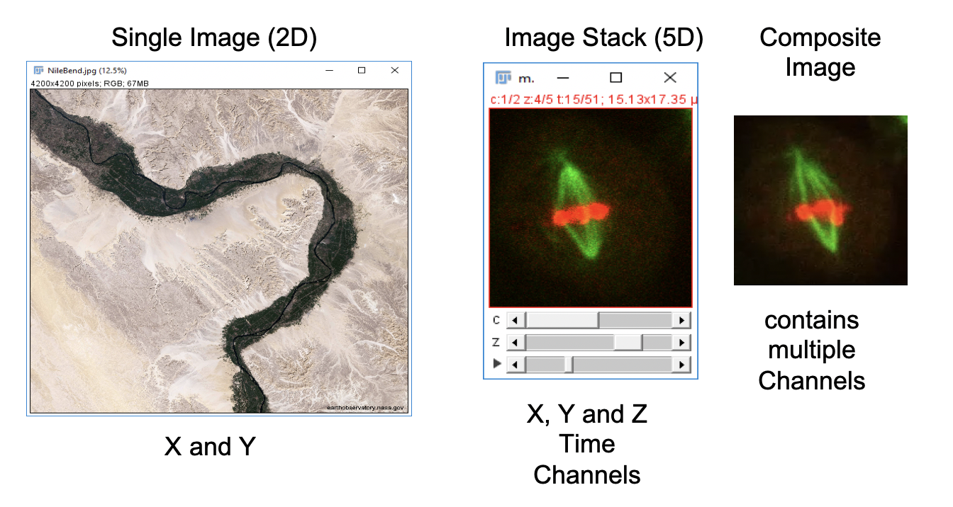
Working with Image Channels

Fiji has built-in tools to manipulate multi-channel composite and RGB images. For this example, open the 5-dimensional (x, y, z, color, time) image stack.

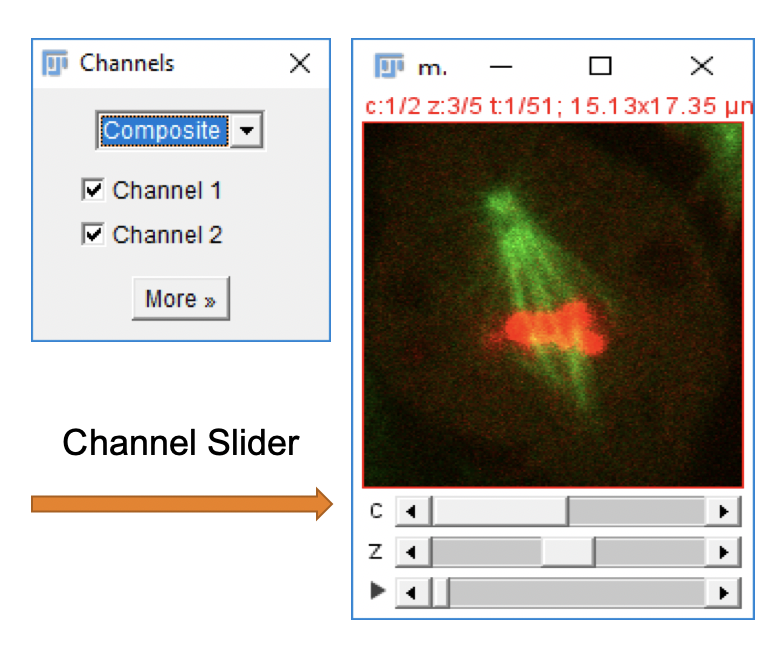
1 Go to File > Open Samples > Mitosis (26MB, 5D stack). An image window should open as shown here.

2 Open the Channels Tool dialog with Image > Color > Channels Tool….

3 In the Channels Tool dialog window, change from Composite to Color. Move the channel slider and note how the display updates based on the selected channel.

4 Switch back to Composite mode. Uncheck selected channels and note how the channel overlay changes based on the selected images.

5 Change to Grayscale. Although the color information has been converted to gray, the pixel intensity values remain unchanged.

6 Change back to Color, Click More >>, select a new color.

7 Change to Composite mode.

Splitting Channels

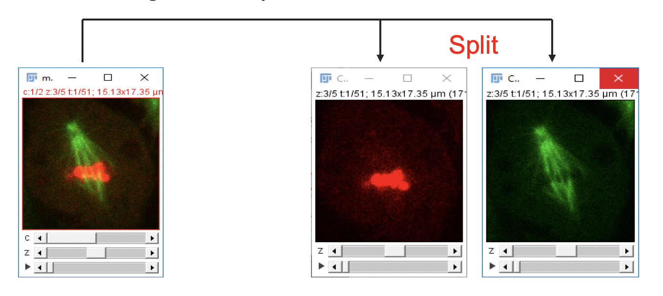
1. Go to File > Open Samples > Mitosis (26MB, 5D stack).

2. Go to Image > Color > Split Channels.

Individual image channels are displayed in separate windows. This operation only works on multi-channel image stacks or RGB images.

Merging Channels

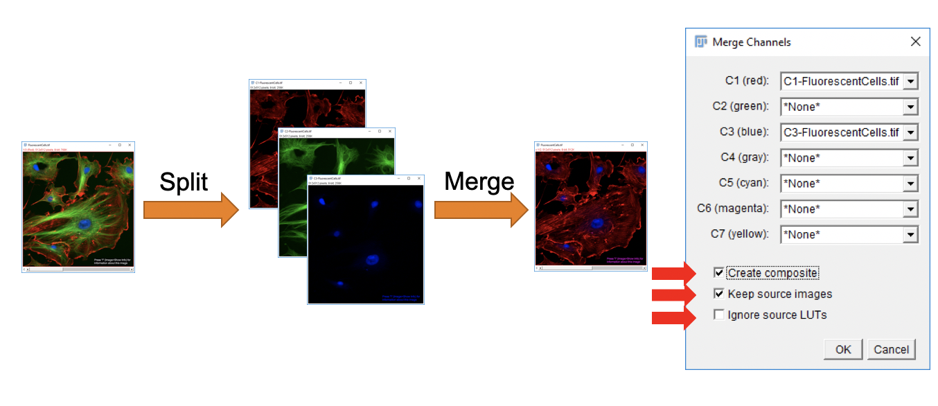
Images displayed in separate windows can be merged into multi-channel composite images. The input images need to be of the same type (either 8-bit or 16-bit pixel encoding). You can merge up to 7 different images into a single multi-channel image.

1. Go to File > Open Samples > Fluorescent Cells.

2. Go to Image > Color > Split Channels.

3. Go to Image > Color > Merge Channels.

4. Set the green channel to None and leave the other default settings. Click OK.

The resulting image should contain a merge of the red and blue channels without the green channel component.

Changing Image Color Assignment

The color representation in 8-bit and 16-bit images is defined by a color Lookup Table (LUT).

For single channel images, you can change the LUT by running these commands:

1. Image > Lookup Tables.

For multi-channel image, you can change the LUT by running these commands:

1. Image > Color > Channels Tools.

2. In the Channels Tools window, switch to Color mode and select a channel of interest.

3. Click More >>, select a new color.

Image Montage and Cropping

Making an Image Montage

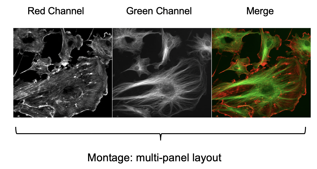
Images can be layed out in a grid-like fashion, aka a montage. Given the regular arrangement of the images in a grid layout, all image tiles used for the montage have to be of the same x-y dimension and same image type (e.g. all 8-bit, 8-bit, 32-bit, or RGB).

The easiest way to create a montage is to create an image stack that contains all the images for the individual image tiles and then use the Fiji Montage tool. Here is an example:

1. Close All Image Windows: File > Close All.

2. File > Open Samples > Fluorescent Cells.

3. Image > Color > Split Channels.

4. Close Blue Image.

5. Select Red Image.

6. Go to Image > Lookup Tables > Grays.

7. Select Green Image.

8. Go to Image > Lookup Tables > Grays.

9. Image > Color > Merge Channels (green and red channel); select Keep Sources.

10. For each of the three images: a) Click on grayscale image window to make it the active window, b) then go to Image > Type > RGB Color.

11. Go to Image > Stacks > Images to Stack.

12. Go to Image > Stacks > Make Montage.(Columns: 3, Scale factor: 1.0)

Image Size: Cropping

Images can be cropped around regions-of-interest (ROIs) that can be drawn with the selection tools in the Fiji Toolbar.

1. Go to File > Open Samples and select any image.

2. Click Rectangular selection icon, then draw rectangular box in image.

3. Go to Image > Crop. This crops image to size of rectangular selection box.

Note that the image will be cropped for all z-focal planes, all channels, and all timepoints.

Image Scale Bars

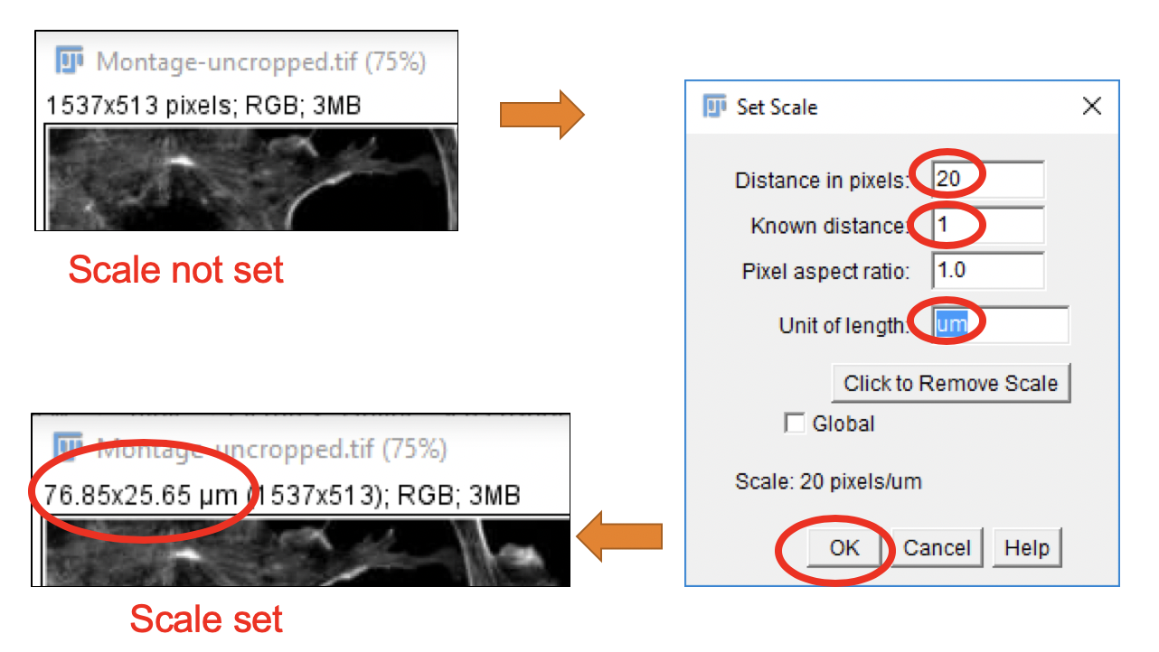
Many scientific instruments used for image acquisition store additional metadata in the image files that contain calibrations defining the size of a pixel (or 3D voxel) for that image or image stack in physical units (e.g. mm, nm, etc.). These values define the scale of an image.

Taking a look at the image window right below the image title indicates whether the image scale (e.g. pixel/voxel size) has been set or not.

• If the scale is not set, the image dimensions are displayed as NNN x NNN pixels, see top left panel.
• If the scale is set, the image dimensions are displayed as NNN x NNN , see bottom left panel.

Defining an Image Scale

You can set or modify an image’s scale following these steps:

1. Go to Analyze > Set Scale....

2. In the top box of the dialog window, enter the number of pixels that correspond to a known physical distance.

3. In the second box, enter the physical distance represented by the pixel distance.

4. Enter the physical units label, e.g. mm, nm, etc.. The label um is interpreted as micrometer.

• If Global is checked, the new scale (or scale removal) operation is applied to all open images.

5. Click OK.

Adding a Scale Bar

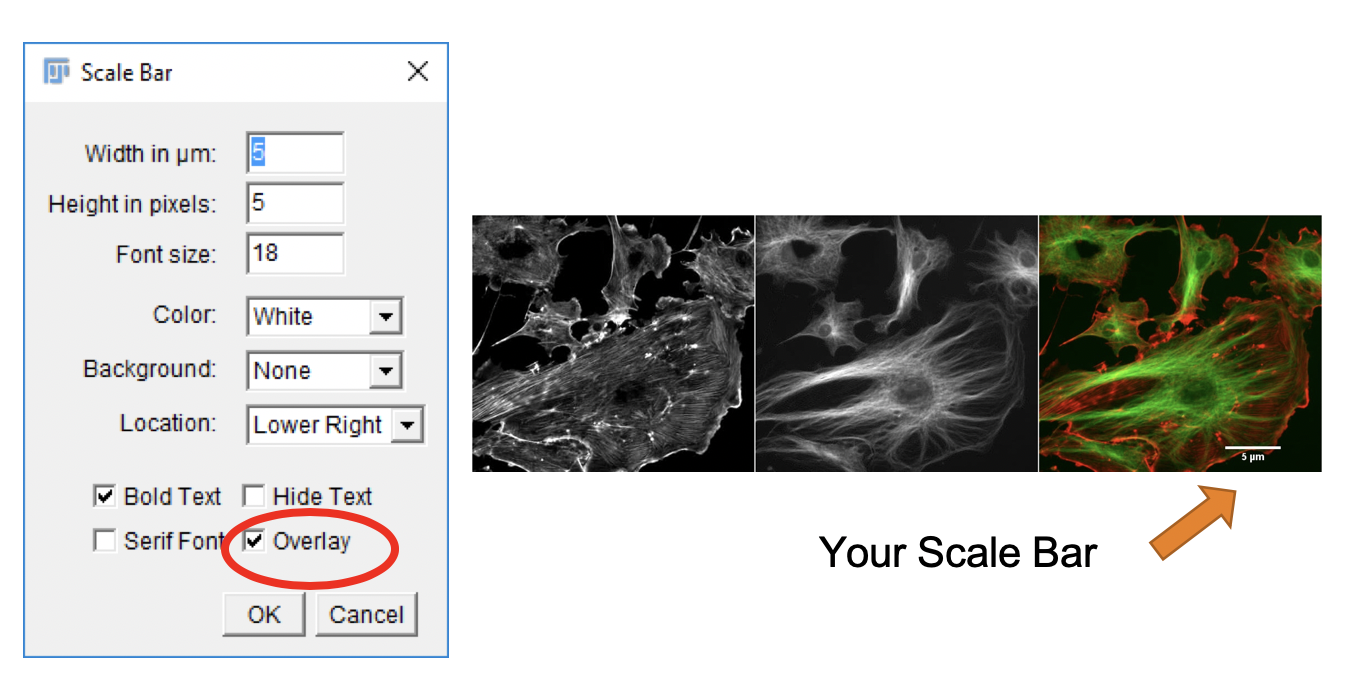
For presentation purposes it is frequently desired to display a scale bar in the image. This can be done following these steps:

1. Go to Analyze > Tools > Scale Bar....

2. Define positioning of the scale bar and its size. Check the Overlay box and click OK.

3. Go to Image > Overlay > Show Overlay/Hide Overlay to toggle between showing and hiding the scale bar.

• The Overlay will not affect the pixel values of the image region under the scale bar. It is non-destructive.

• Saving the image in TIF format retains the non-destructive overlay.

• Saving the image in JPG format burns the overlay into the image.

Useful ImageJ/Fiji Keyboard Shortcuts

Shortcut	Operation
Ctrl + I	Show image file info
Ctrl + Shift + D	Duplicate current image
Ctrl + Shift + X	Crop image
Ctrl + Shift + I	Invert image
Ctrl + A	Select All (entire image)
Ctrl + Shift + A	Deselect marked region
Ctrl + M	Measure (in selected region)
Ctrl + T	Add selection to ROI Manager

*On a Mac, use the Command key instead of the Ctrl key.

Image Filtering & Enhancement

Applying Filters: Noise Removal

Image noise is an undesirable by-product of image capture that adds spurious and extraneous information.

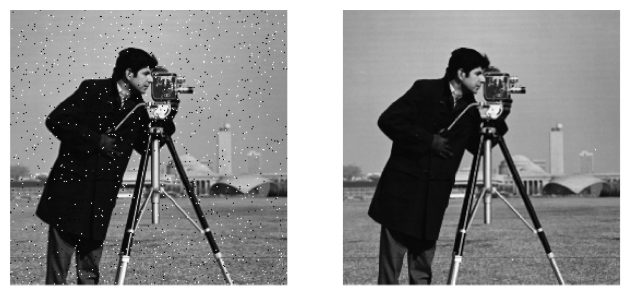
How Do Filters Work?

Fiji provides several standard filters that can be applied to images. Here we are just exploring a few of them.

1. Open image file noisy_image.tif from the Tutorial Example Files.

2. Create three copies of the image file by pressing Ctrl + Shift + D (three times).

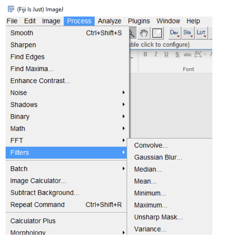
3. Go to Process > Filters and experiment with the Mean, Median, Gaussian, and Unsharp Mask filters on the four images.

4. Experiment with settings and click Preview.

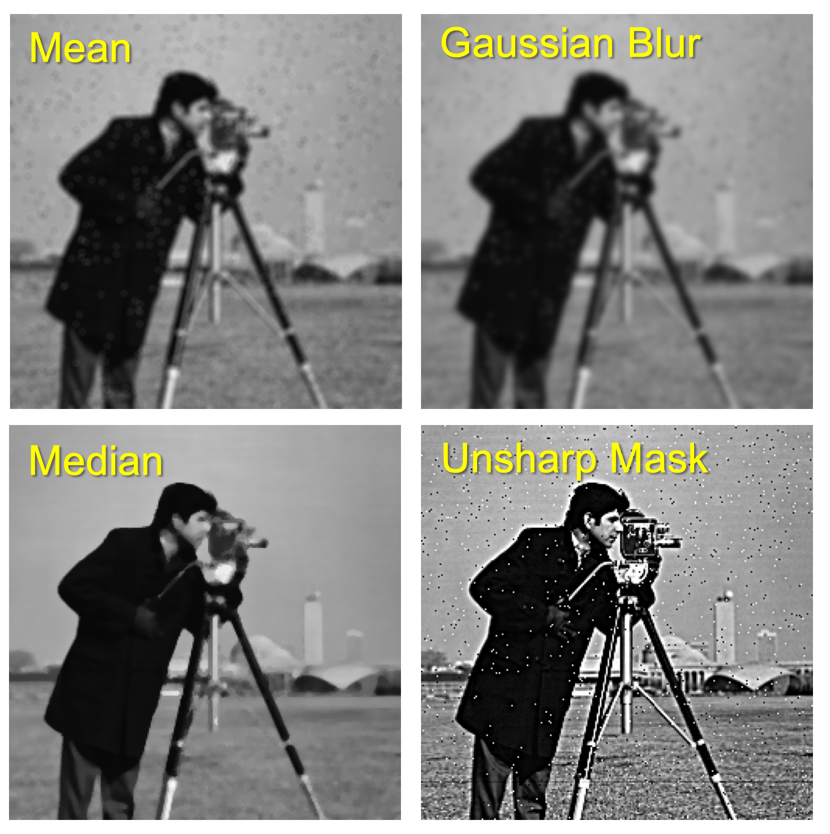
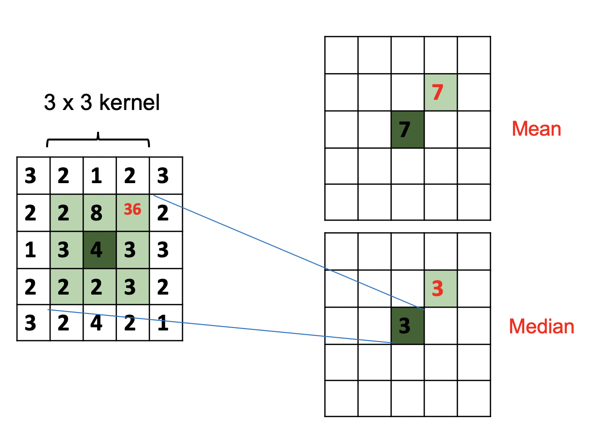
Comparing Average (Mean) and Median Filters

• Mean: Replaces pixel value with average value in kernel region.

• Median: Replaces pixel value with median value in kernel region.

Other Commonly Used Filters

Filter	Effect
Convolve	Convolution with custom filter
Gaussian Blur	Gaussian filter, reasonable edge preservation
Median	Median of neighbors, non-linear, good for salt-and-pepper noise reduction
Mean	Average of neighbors, smoothing
Minimum	Smallest value of neighbors, smoothing
Maximum	Largest value of neighbors, smoothing
Variance	Variance of neighbors, indicator of image textures, highlight edges

Removing Periodic Noise (Advanced)

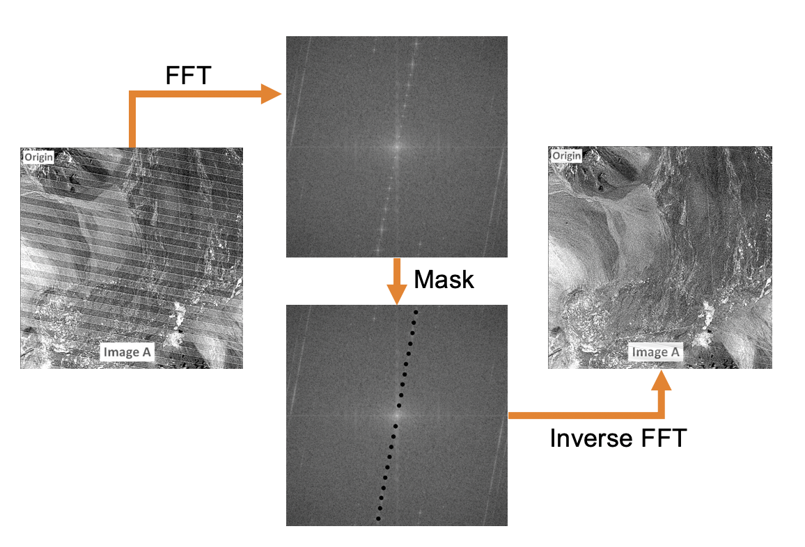
Periodic noise as shown by the banding pattern observed in this image cannot be removed with the kernel-based standard filters described above. However applying Fast-Fourier Transform (FFT) analysis can reveal the periodicity of such noise represented by the high intensity spots in the the FFT image (top middle panel). By masking these hotspots (bottom middle panel) and applying the inverse FFT one can retrieve the original image without the periodic noise (right panel).

Applying Filters: Edge Detection

Edge detection is commonly used to define the outline of objects of interest. It is implemented by applying special convolution kernels.

Note that edge detection algorithms can be very sensitive to noise. So it is generally advised to remove noise with other filters first (e.g. median filter which preserves edges quite well) before applying the edge detection filter (see images below).

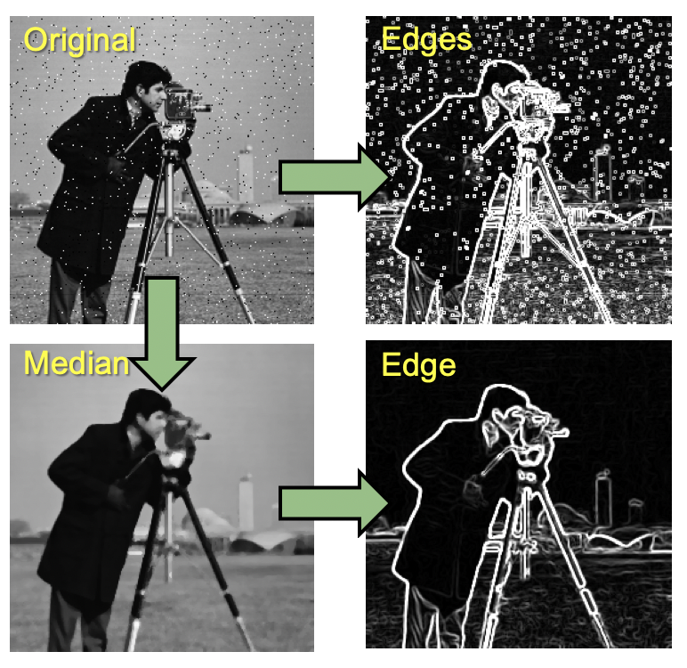
Image Segmentation

• Image Segmentation is the process that groups individual image pixels that represent specific objects.

• It often involves the application of a variety of image pixel filters.

• It requires binary (black and white) image masks and object shape descriptors (morphometric parameters).

Example: Blob Analysis

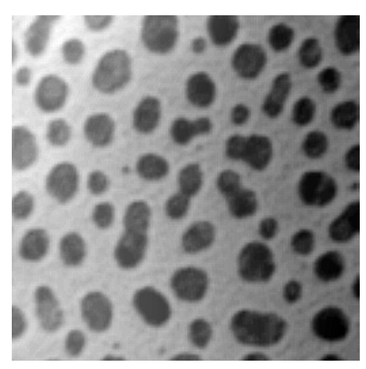
To illustrate typical steps in image segmentation and analysis, we are going to process the blobs-shaded.tif image that is part of the [Tutorial Example Files] (#example-files).

Analysis Goals:

• Separate dark spots as individual objects from background.

• Reject small objects (debris) by size exclusion.

• Count total number of objects and compute average object size.

• Measure size (2D surface area) of each object.

Separating “Blobs” from Background

In order to separate the dark spots from the background we will be using intensity thresholding. The idea is that all pixels with an intensity below (or equal) the threshold go in one bin, all other pixels go into another bin. Pixels in one bin are considered to belong to objects of interest while those in the other bin are considered background. This is the principal method to create binary images.

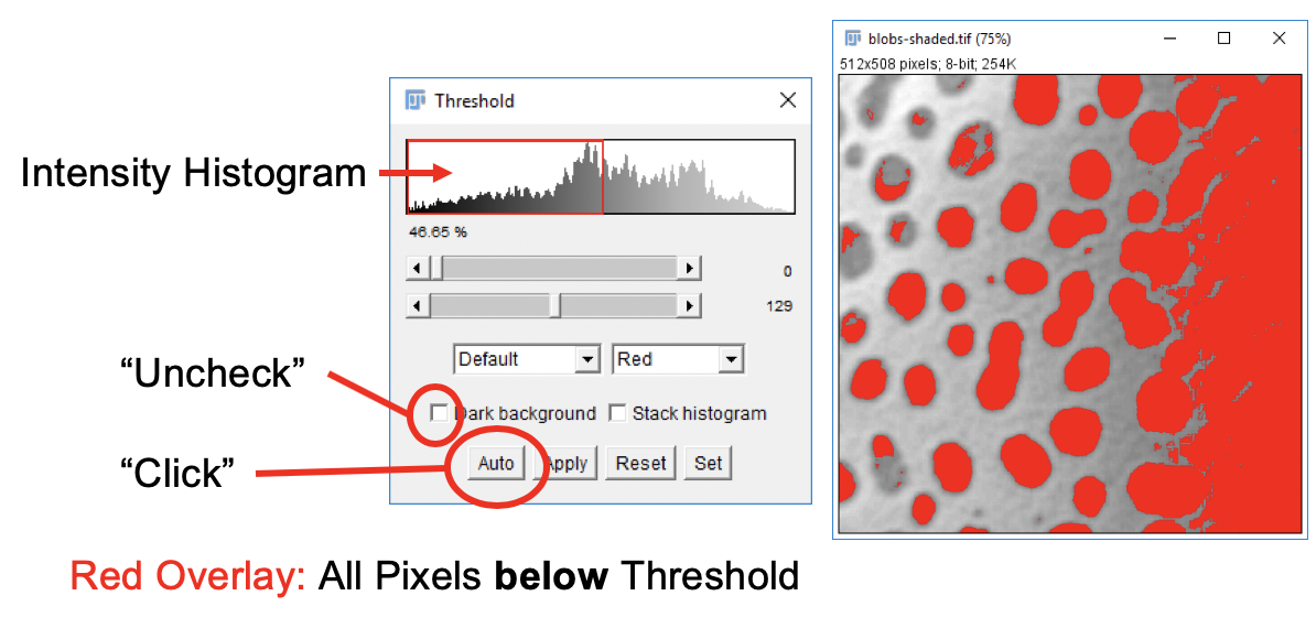
1. Open image file blobs-shaded.tif.

2. In menu, go to Image > Adjust > Threshold….

3. Click on image window, then click on Auto button in Threshold window. If you lost track of the Threshold window, goto Windows and select it from the list.

4. In the Threshold dialog window, uncheck the Dark Background box. In the drop-down boxes select Default and Red.

5. Move the sliders and observe the change of the red pattern overlaying the image. Click Reset to remove the overlay. Don’t click Apply yet!

• What is the problem?

Correction of Uneven Background Signal

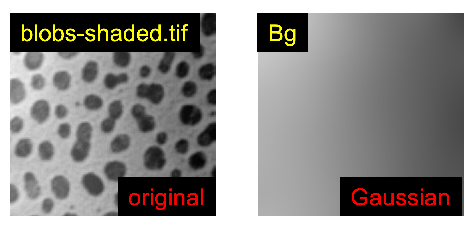
A Background Correction Image

1. Go to Image > Duplicate, in the Title box enter: Bg.

2. Go to Process > Filters > Gaussian Blur….

• Check the Preview box.

• Try different Sigma Radius values: e.g. 1, 20, 100.

3. Finally, set Sigma Radius to 60.

4. Click OK.

Performing the Background Correction

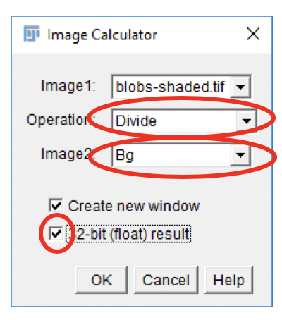
5. Go to Process > Image Calculator….

• From the Image1 drop-down, select the blobs-shaded.tif image.

• Select the Divide Operation.

• From the Image2 drop-down, select the Bg image.

• Check the Create new window box.

• Check the 32-bit (float) result box.

• Click OK.

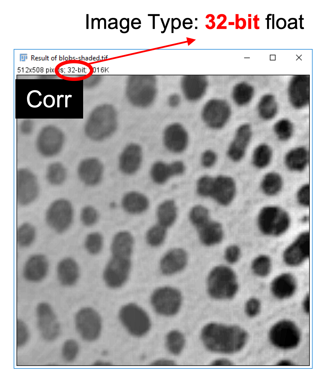
6. Click on the resulting window that contains the corrected image.

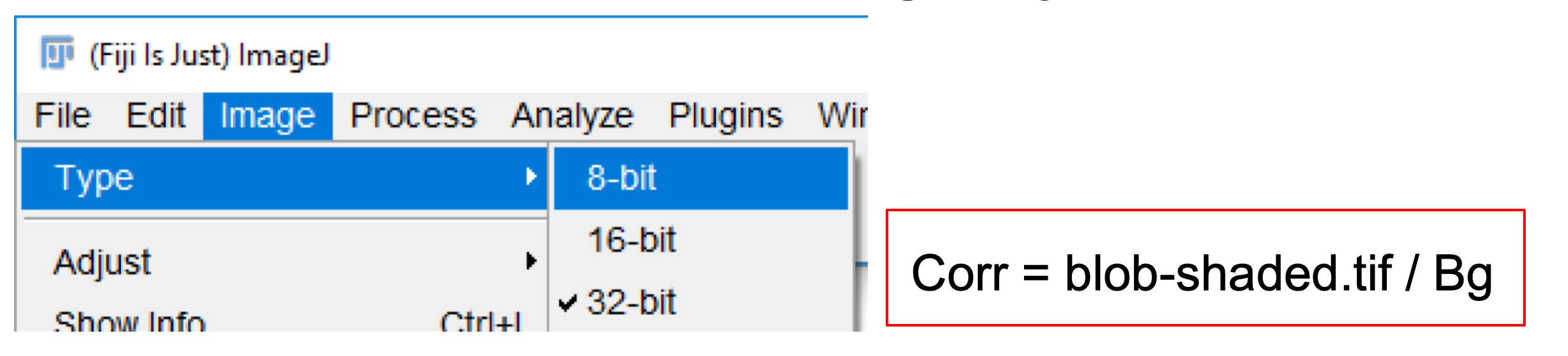
7. Go to Image > Rename... and enter Corr as a new name for the corrected image.

8. Go to Image > Type > 8-bit to change the image from 32-bit float to 8-bit integer encoding.

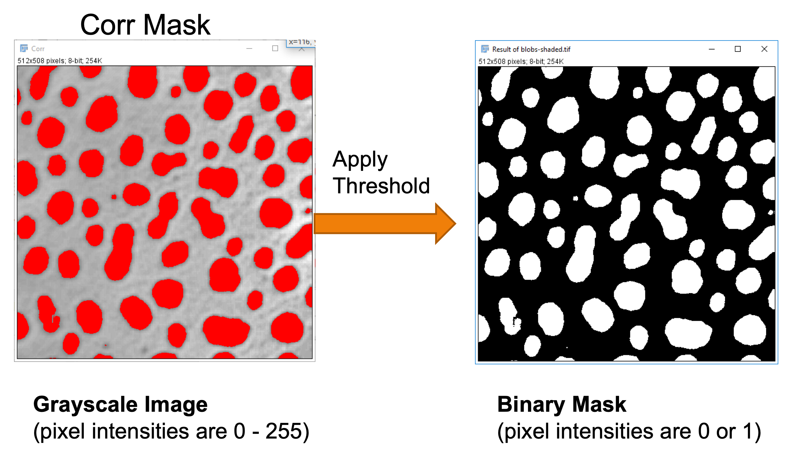
Creating a Binary Object Mask

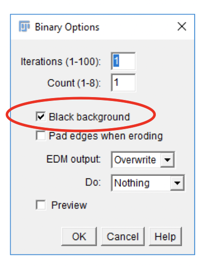
9. Go to Process > Binary > Options. Check the Black background box and click OK. This controls the display mode of thresholded images and also the mode that the Particle Analyzer uses to identify objects (see below). In our example objects of interest will be displayed white on black background.

10. Go to Image > Adjust Threshold.

• In the Threshold dialog window, choose the Default algorithm.

• Choose the Red overlay.

• Deselect Dark Background and deselect Stack histogram.

• Click on the Corr image window and click Auto in the Threshold window. Note the uniform detection of dark spots indicated by the red overlay. Note the bimodal distribution of the pixel intensity values in the thresholding histogram. Compare this thresholding to the one obtained for the original image blobs-shaded.tif.

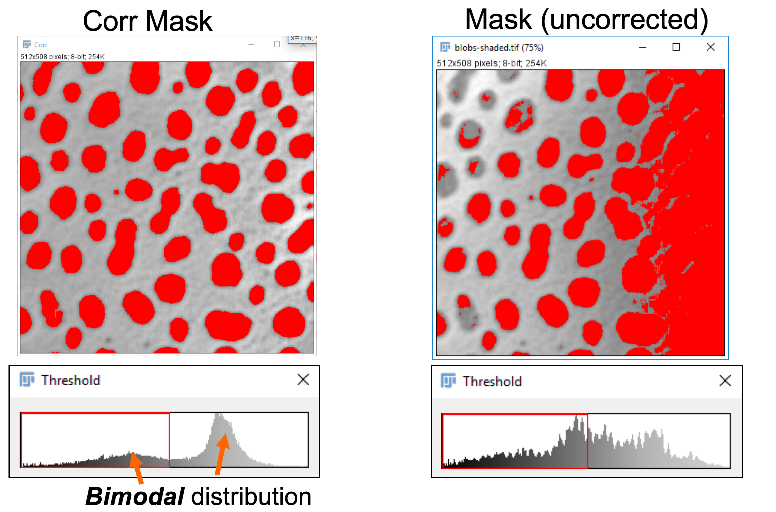
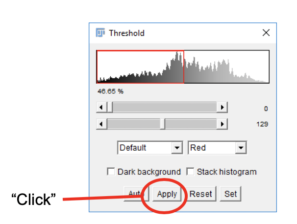
11. In the Threshold dialog window, click Apply.

• If you see a message like: “Convert to 8-bit mask or set background pixels to NaN”, it means that you are running the thresholding on a 32-bit image. Convert the Corr image to 8-bit first (see step 8).

• If you see black objects on white background, check Process > Binary > Options (step 9).

• Redo the thresholding on “Corr” image.

12. Go to Image > Rename and enter Mask as a new image title.

The result after steps 1-12 should be a binary mask image that shows white bobs on a black background.

Splitting Joined Objects

The previous steps produced a binary mask, but closer inspection reveals that some blob objects are fused. These appear as peanut-shaped objects. We will apply a watershed algorithm to separate these fused objects.

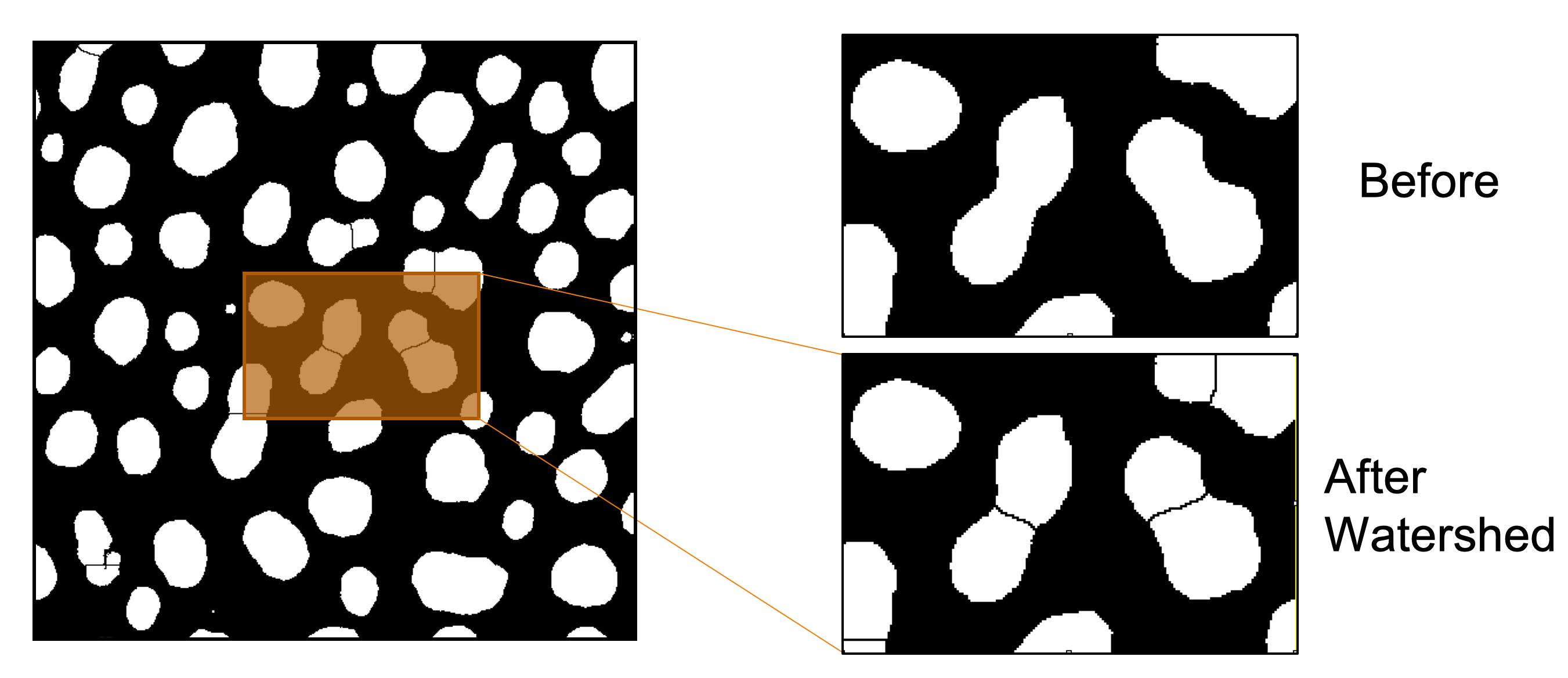
13. Click on the Mask image window and go to Process > Binary > Watershed.

14. Save the image obtained after the watershed operation as blobs-watershed.tif.

• The watershed algorithm only works on binary images, e.g. the black and white “blob” mask.

• It only works for objects that show significant opposing convex-to-concave curvature (neck regions).

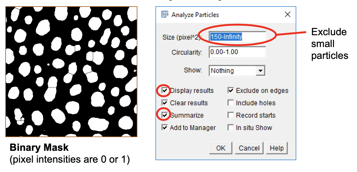
Analyze Particles

Now we are ready to identify and extract information from each blob.

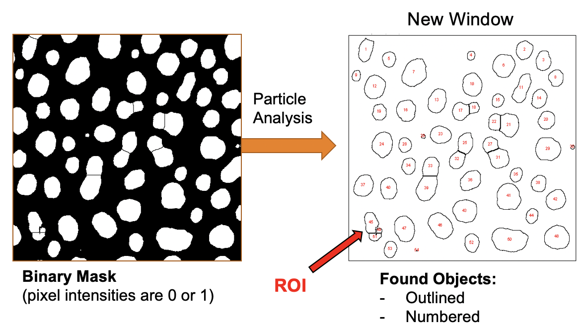
15. Go to Analyze > Analyze Particles....

• In the Analyze Particles dialog, set up the analysis parameters as shown.

• Click OK.

The option Show Outlines leads to the creation of a new image that contains the outline and object ID (red numbers).

The option Add to Manager sends the definition for each identified particle, i.e. dark blob, to the Region-of-Interest Manager, (ROI Manager for short).

The ROI Manager

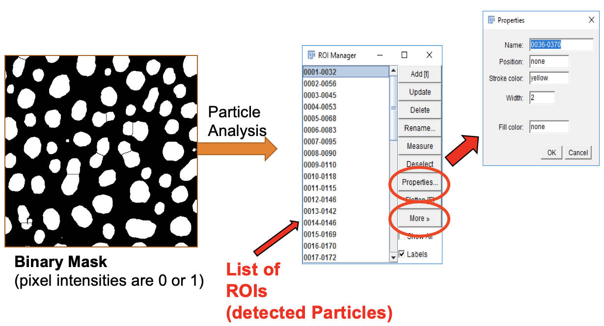
Regions-of-interest (ROIs) define groups of pixels in an image. ROIs can have different shapes, e.g. line, rectangular, ellipsoid, polygonal, text, or irregular. An ROI can be used to

• Measure pixel values in a specific image region.
• Change pixel values in a specific image region.
• Mark image regions in non-destructive overlays (without changing pixel values).

When we use the Particle Analyzer with the Add to Manager option, the ROI for each blob is sent to the Roi Manager.

ROI Properties

Via the Properties button, the ROI Manager provides functions to change propoerties of selected ROIs, e.g. name, Z-position, outline color & width, and fill color. Multiple ROIs can be selected by holding the Ctrl (command on a Mac) or Shift keys while clicking on the ROIs.

ROI Import & Export

The ROI Manager can save selected ROIs to a file or open ROIs from a file. Typically, the ROI files have a .roi or .zip extension. The Open & Save functions are available after clicking the More>> button in the ROI Manager.

• Save: Export All Selected ROIs to File

• Open: Import ROIs from ROI file

• This only affects selected ROI.

• If no ROIs are selected, new properties are be applied to all ROIs in Manager.

Image Object Measurements

Set Measurements

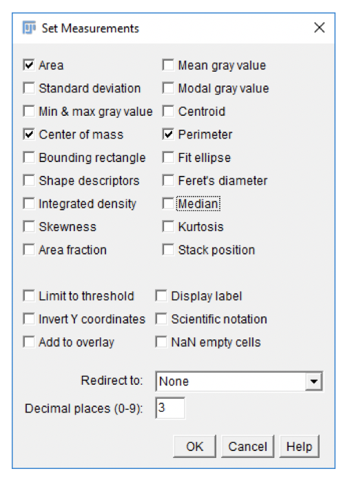
Fiji can measure a variety of parameters for each region-of-interest, or an entire image. The specific measurements to be calculated by the Particle Analyzer can be set in the Set Measurements dialog.

1. Go to Analyze > Set Measurements....

• Adjust settings as shown in screenshot. Click OK.

• Settings affect future measurements, not existing ones.

2. For quick measurements, draw a selection on the image and press Ctrl + M.

• Measurements occur for current selected region in the current image.

Example:

1. Draw a selection on image

2. Use Ctrl + M.

3. Change settings in Set Measurements window.

4. Use Ctrl + M.

5. Select an ROI in the ROI Manager. Click Measure or use Ctrl + M to create measurements for the currently selected ROI.

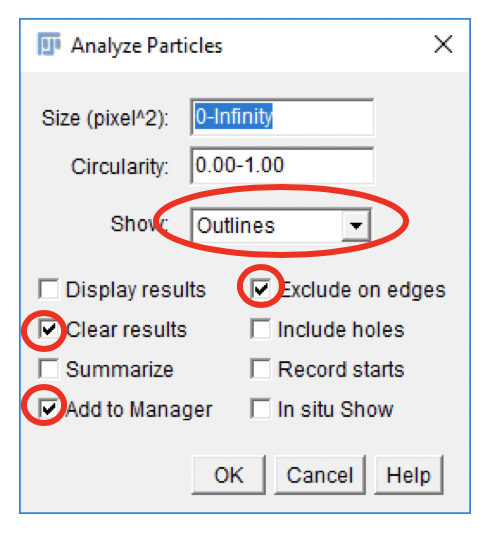
Analyze Particles with Custom Parameters

The Particle Analyzer allows filtering of identified ROIs by size and circularity (range 0.0-1.0). A perfect circle has a circularity of 1.0. Let’s filter the identified blobs and discard any ROI that has an area <150 square pixels.

1. Go to Edit > Selection > Select None (Ctrl + Shift + A).

2. Go to Analyze > Analyze Particles....

3. In the Analyze Particles dialog window, set up the analysis parameters as shown in the screenshot.

4. Click OK.

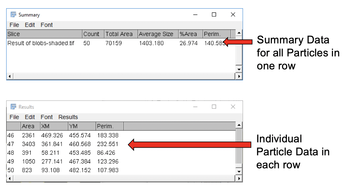
Based on our selection, the Particle Analyzer creates two results tables, titled Results and Summary. The type of measurements computed (e.g. Mean, Median, etc.) depend on the settings in the Set Measurements dialog.

• Each line in the Results table reflects measurements for a single ROI.

• The Summary table, as the name implies, provides summary statistics for all ROIs.

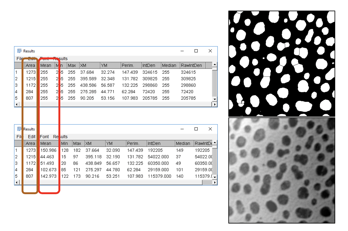
Measuring Pixel Intensities

Let’s go back and modify the measurement selection.

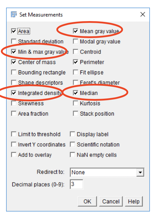
1. Go to Analyze > Set Measurements....

2. In the Set Measurements dialog window, set up the analysis parameters as shown in the screenshot.

3. Click OK.

4. Select all ROIs:

• Go to Window > ROI Manager.
• Click on first ROI, hold Shift key,
• Scroll down, click last ROI in list.

5. Measure ROIs in the Mask image

• Click on black/white mask image
• In ROI Manager window, click Measure. This adds measurements for all selected ROIs to the Results table.
• Click on the Results window, go to File > Rename, and enter Mask-Results as a new name.
• If you don’t rename the window, the Results will be overwritten by new measurements.

6. Measure ROIs in the original image

• Click on blobs-shaded.tif image
• In ROI Manager window, click Measure. This adds measurements for all selected ROIs to the Results table.

Now we can compare the intensity measurements for the corresponding ROIs in the Mask and the blobs-shaded.tif images.

• What do you observe?

Additional ROI Manager Functions

• ROIs that are listed in the ROI Manager window can be saved to a file (single ROI or multiple ROIs).
• Conversely, ROIs can be loaded from file into the ROI Manager and (re-)applied to an image.
• Hand-drawn ROIs created with the ROI tools can be added to the ROI-Manager.
• ROIs can be renamed and colored.
• ROIs can be combined to create ROIs with complex shapes.

Go to the Exercises section for ideas to explore ROI-Manager functionality.

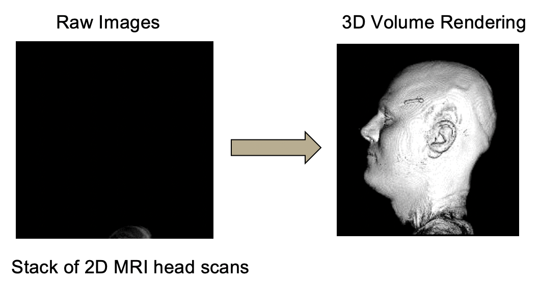
3D Image Reconstruction

Isolating the Brain Segmentation

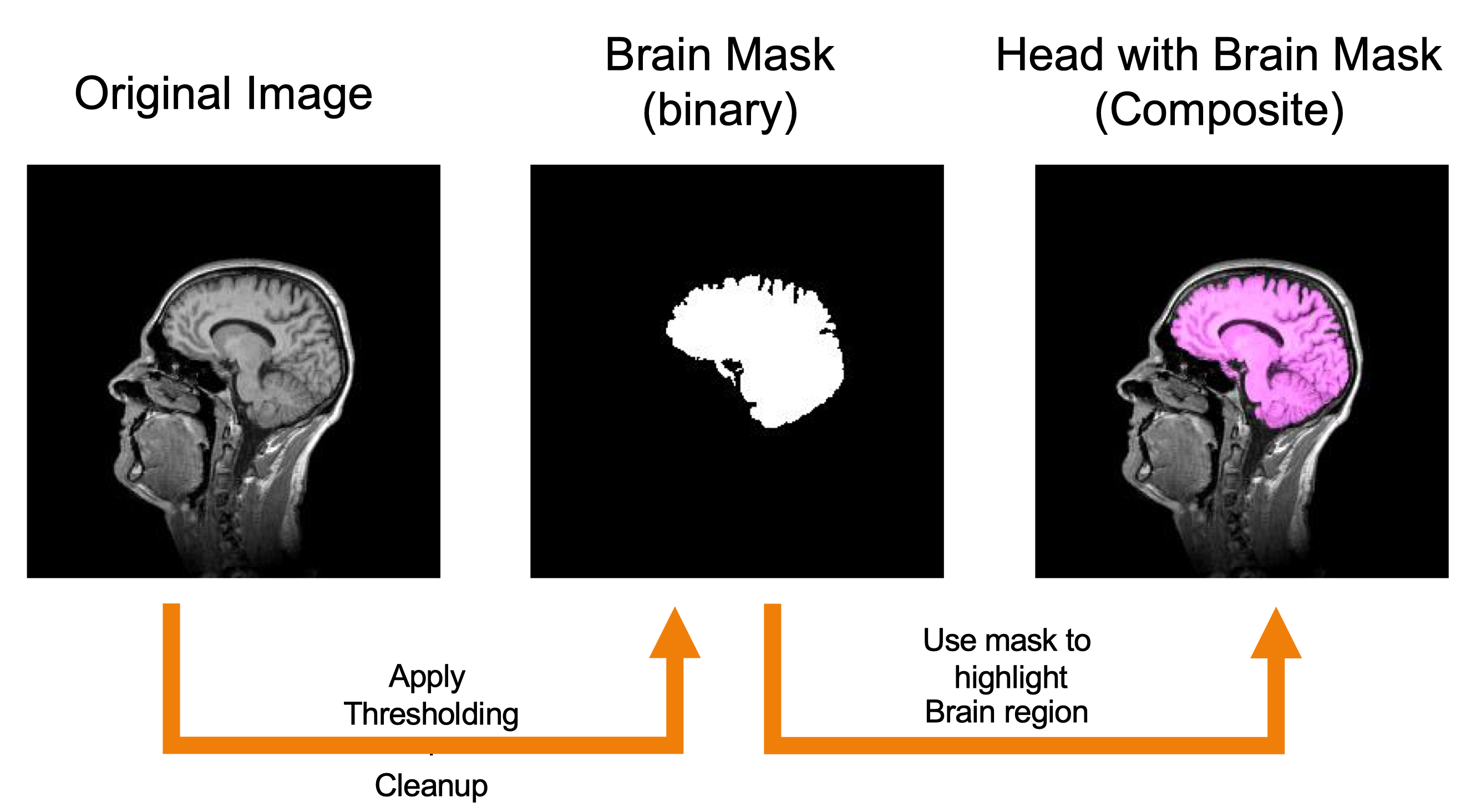
Creating the Brain Segmentation

1. Apply gaussian filter (0.5).

2. Apply local thresholding (Grey Median, Otsu).

3. Run particle analysis (1000-infinity particle size).

4. Manual clean up segmentation mask as needed.

5. Save brain segmentation mask as TIF image stack.

These steps have been executed for you. The resulting brain segmentation mask is saved as brain-mask.tif in the Tutorials Example Files.

Creating the Composite 3D Rendering

1. Go to File > Open Samples > T1-Head.

2. Go to Image > Type > 8-bit.

3. Go to File > Open and select brain-mask.tif see Tutorials Example Files.

4. Go to Process > Image Calculator:

• Select t1-head.tif as Image 1.
• Select the AND operation.
• Select brain-mask.tif as Image 2.
• Check the Create new window box.

This will create a new grayscale window with the brain proper that corresponds to the mask.

5. Go to Image > Color > Merge Channels: t1-head.tif (gray), brain (magenta)

6. Go to Plugins > 3D Viewer.

• Select Display as Volume. Leave the other default settings.

8. In 3D Viewer, go to Edit > Change Transparency: Change skull transparency to 75%.

9. Go to View > Create 360 degree animation to view a rotating animation of the rendered head volume.

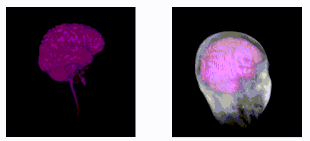
• Better: Export surfaces in Fiji to .stl files.

• Process .stl surfaces for high quality rendering in other software, e.g. Paraview, Blender, etc..

Fiji/ImageJ Tutorials and Resources

https://imagej.nih.gov/ij/docs/examples/

Exercises

1. Saving files in different file formats

Fiji supports many different file formats.

1. Use File > Open Samples to open an image of your choosing

2. Go to File > Save As and pick a file format to export the current image to.

Note that some image file formats use compression algorithms that may reduce the pixel resolution or dynamic range of an image’s intensity values. The TIF file format is very versatile because it can store image data without resolution loss, it can handle multi-image files (i.e. image stacks or multi-page), store image annotations as file internal metadata, and can be read by many programs. File import/export functionality is further extended by the Bio-Formats plugin (Plugins > Bio-Formats). See https://docs.openmicroscopy.org/bio-formats/6.0.0/

2. Image Channels

2.1 Splitting and Merging Channels

1. Go to File > Open Samples > Mitosis (26MB, 5D stack).

2. Go to Image > Color > Split Channels.

3. Go to Image > Color > Merge, merge the two channels but assign new colors to each channel.

What happens if you assign one of the images to multiple different colors?

2.2 Manipulating Color Lookup Tables

Color lookup tables (LUTs) can be used on 8-bit grayscale, 16-bit grayscale, and 8-bit Color images. Note that 8- bit color is not the same as RGB color. LUTs for 16-bit grayscale will be resampled to 8-bit (256 colors).

1. Go to File > Open Samples > Clown

2. Go to Image > Zoom > In.

3. Go to Image > Color > Edit LUT.

Did this work? Look at the image information in the clown.jpg window. Alternatively, go to Image > Show information and look at the Bits per pixel entry. What is the image format?

4. Click on the clown.jpg image and convert the image to 8-bit color (Image > Type > 8-bit Color) Keep 256 colors (the default). Click OK.

5. Go to Image > Color > Edit LUT. The window shows the LUT color palette

6. Double click on a LUT tile and edit its RGB values to pure blue. Click OK and repeat this for other LUT entries, change the color representation as you wish.

What do you observe?

3. Image Montage

For this exercise we are creating a montage of RGB images, each image representing the center focal plane at a single timepoint within an x-y-color-t timelapse series. Experiment with creating different image tile sizes and border widths.

1. Close all images (File > Close All).

2. Go to File > Open Samples > Mitosis (26MB, 5D stack).

3. Go to Image > Type > RGB Color. Keep all slices and frames selected.

4. Go to Image > Duplicate. Check the Duplicate Hyperstack box, enter Slices (z): 3 (central focal plane), enter Frames (t): 1-51. Click OK.

5. Click on the newly created stack. It should contain images for a single focal plane over multiple timepoints (frames).

6. Save this image stack as a TIF file to your hard drive so you can create new montage layouts without having to go through steps 1-5 again.

7. Go to Image > Stacks > Make Montage. In the dialog box set the following values:

• Columns: 10
• Rows: 6
• Scale factor: 0.25
• Border width: 5
• Check Use foreground color

8. Click OK.

Select the image stack created in step 5 (or reopen the stack saved in step 6) and create new montages with modified montage settings. To change the foreground color for the border, double click on the Color Picker in the Fiji toolbar.

4. Image Scale Bars

Scale bars can be added to any image. Before a scale bar can be drawn, the pixel size has to be defined.

1. Go to File > Open Sample and select an image.

2. Repeat step 1 and open a second image.

3. Go to Analyze > Set Scale.

4. If the image does not have a scale bar, the entries for Distance in pixels and Known distance will be set to zero values and Scale label will show at the bottom the dialog box.

5. Change the values for Distance in pixels and Known distance to non-zero values. Leave the Global box unchecked.

6. Enter a value for Unit of length. This can be any character sequence. If you enter “um” (without the quotes) the unit will be set to μm.

7. Click Ok.

Look at the active image window (currently in front). The scale is indicated below the window title. The scale of the second window should remain unaltered.

8. Go to Analyze > Set Scale again.

9. Change the Distance in pixels, Known distance, and Unit of length values.

10. Check the Global box.

11. Click Ok.

Note that the scale has changed for all open images. To remove a scale bar from an image, go to Analyze > Set Scale and press the Click to Remove Scale button. If the Global box is checked, it will remove the scale on all open images, otherwise the scale will be removed for the current image only.

5. Custom Image Filters

To apply a filter to images, a convolution kernel has to be created. The built in filters have standardized convolution kernels. You can create your own convolution kernels to create custom filters. In this example we create a simple edge detector, called the Sobel operator.

1. Open the noisy.tif image.

2. Apply a filter to remove the salt-and-pepper noise, e.g. with the median filter.

3. Duplicate the image.

4. Go to Process > Filters > Convolve.

5. In the textfield of the dialog box, enter these numbers (each number separated by a white space).

-1 0 1

-2 0 2

-1 0 1

6. Check the Preview box. Experiment with changing the kernel values; make sure to keep the square matrix format.

7. Click OK. What edges are highlighted in the image? Can you modify the kernel to detect the missing vertical edges?

8. Create another kernel with these values and apply it to the copied image obtained in step 3:

-1 -2 -1

0 0 0

1 2 1

What edges are being detected now?

9. Go to Process > Image Calculator.

10. Select the output image from step 7 as Image 1.

11. Change Operation to Max.

12. Select the output image from step 8 as Image 2.

13. Check the Create new window box.

14. Check the 32-bit (float) result box.

15. Click OK.

The resulting image should show a combination of edges detected in steps 7 and 8. Can you create four kernels to detect all vertical and horizontal edges?

6. Image Segmentation & Object Measurements

For this exercise we assume that we already have a binary mask (thresholded) image, and we will use the Particle Analyzer for image segmentation and object measurements.

1. Open the blobs-watershed.tif image. This should be a binary image.

2. Go to Analyze > Set Measurements and change the selection of measurement options.

3. Go to Analyze > Analyze Particles and modify the Size (pixel^2), Circularity (1.0 refers to perfect circular shaped objects), and Show options.

4. Click OK.

5. Repeat steps 2-4 and experiment with different settings.

Depending on your selection you will see a results table with data for each detected object (if Display results is checked), a summary table for all results (if Summarize is checked), and the ROI-Manager (if Add to Manager is checked) with a list of ROIs corresponding to the individual objects.

6. Go to File > Open Samples > Blobs.

7. Click on the blobs-watershed.tif image.

8. Go to Analyze > Set Measurements, check the Min & max gray value and the Mean gray value boxes, and change the Redirect to option to blobs.gif. This means that object detection is performed on the blobs-watershed.tif binary mask, but pixel intensity measurements will be performed on the blobs.gif image due to the redirect.

9. Go to Analyze > Analyze Particles. Click OK.

Repeat the measurement results with and without redirect and compare the changes in the results for Min & max gray value and the Mean gray value.

7. ROI Manager

The ROI Manager is very useful to handle multiple ROIs. It allows saving/loading ROIs and also to combine simple shaped ROIs into more complex ones.

1. Open an image of your choice.

2. Use any of the selection tools from the Fiji toolbar to draw a selection area onto the image.

3. Go to Selection > Edit > Add to Manager. This will add the current selection to the ROI Manager.

4. Draw a new region of interest and go to Selection > Edit > Add to Manager.

7.1 Saving ROIs to file

The ROI Manager should show two ROIs.

5. In the ROI Manager, click on one of the ROIs.

6. In the ROI Manager, click More» and then Save. In the dialog box enter a name for the ROI file and click Save.

7. In the ROI Manager, hold the Shift key and select both ROIs.

8. Click More» and then Save. In the dialog box enter a name for the ROI file and click Save. This will save multiple ROI definitions into a single file.

Notes:

• For a single ROI, the default ROI file extension is .roi. For multiple ROIs, the default file extension is .zip.

• If none of the ROIs are selected, the operations in the ROI Manager are applied to all ROIs.

7.2 Opening ROIs from file

1. In the ROI Manager, select all ROIs and click Delete.

2. Click on More» and then click Open. Select the ROI file saved under exercise 7.1 step 8 (multiple ROIs).

3. Click on one of the ROIs in the ROI Manager. This should create corresponding selection in the current image.

Note: You can open another image and reload saved ROIs to apply them to the new current image.

7.3 Changing ROI display properties Each ROI has multiple properties, e.g. position, color, etc.

1. In the ROI Manager, select the first ROI (or reload from file).

2. Click on Properties.

3. Change the Name to ROI_1, the Stroke color to blue, and the width to 2. Click OK.

4. Select the second ROI.

5. Click on Properties.

6. Change the Name to ROI_2, the Stroke color to red, the width to 1, and the Fill color to cyan. Click OK.

7. Click OK.

If you have multiple ROIs selected OR none at all, the properties will be applied to all ROIs.

7.4 Combining ROIs

Simple ROI shapes can be combined into more complex ones.

1. In the current image, draw a new selection that partially overlaps the first ROI.

2. Add the selection to the ROI Manager. It should show as the last one in the ROI Manager list.

3. In the ROI Manager, hold the Ctrl (Windows) or Command (Mac) key and click on the first and third ROI.

4. A context menu should pop up; if not, click on More ». In the ROI Manager’s context menu, select OR (Combine). The menu will disappear. In the ROI Manager, click on Add [t] button. A new ROI will appear at the bottom of the ROI Manager list.

5. Select the last ROI in the list (the one you just created). It encompasses the combined area of the first and third ROI.

6. Repeat steps 3 and 4 but choose different ROI combination methods, e.g. And, XOR. The And operation produces a new ROI that contains only the overlapping region of the selected ROIs, while the XOR operation creates a combined ROI that excludes any overlap between the selected ROIs.