Building a Simple Neural Network

Neural Network Construction

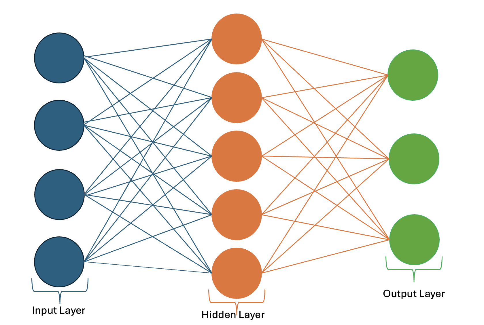
A neural network consists of multiple layers, each performing specific transformations on the input data.

Frequently used Layers in PyTorch:

import torch.nn as nn

fc_layer = nn.Linear(in_features=128, out_features=64)      # Fully Connected Layers

conv_layer = nn.Conv2d(in_channels=3, out_channels=32, kernel_size=3, stride=1, padding=1)  # Convolutional Layers

rnn_layer = nn.RNN(input_size=10, hidden_size=20, num_layers=2, batch_first=True) # Recurrent Layer

dropout_layer = nn.Dropout(p=0.5)

bn_layer = nn.BatchNorm1d(num_features=64)

maxpool_layer = nn.MaxPool2d(kernel_size=2, stride=2)

avgpool_layer = nn.AvgPool2d(kernel_size=2, stride=2)

layer_norm = nn.LayerNorm(normalized_shape=128)

Variations:

• nn.Conv1d, nn.Conv2d, nn.Conv3d
• nn.LSTM → Handles long dependencies.
• nn.GRU → Simpler alternative to LSTM.
• nn.BatchNorm1d, nn.BatchNorm2d, nn.BatchNorm3d
• nn.Dropout1d, nn.Dropout2d, nn.Dropout3d
• nn.MaxPool1d, nn.MaxPool2d, nn.MaxPool3d
• nn.AvgPool1d, nn.AvgPool2d, nn.AvgPool3d
• nn.AdaptiveAvgPool2d → Fixed output size pooling.
• nn.LayerNorm, nn.InstanceNorm2d

---

Building a Model and Forward Propagation

There are two ways to define a neural network, the Sequential Class and the Module Class.

Defining a Model with the Sequential Class

The Sequential class is a PyTorch object used to simplify the creation of NN. It allows stacking layers sequentially in the order they are defined without explicitly writing a forward() method. It’s best used for simple models or prototyping.

import torch.nn as nn

model = nn.Sequential(
    nn.Linear(784, 128),  # Input Layer
    nn.ReLU(),            # Activation Layer
    nn.Linear(128, 64),   # Hidden Layer
    nn.ReLU(),            # Activation Function
    nn.Linear(64,10)      # Output Layer
)

Defining a Model with the Module Class

The Module class is the base class for all NN in PyTorch. It provides a framework for defining and organizing the layers of a neural network and enables easy tracking of parameters, gradients, and training. The Forward function defines how the input data is processed through the layers. The .parameters() method (inherited from the Module class) returns the model parameters and is essential for training.

import torch.nn as nn
class SimpleModel(nn.Module):
    def __init__(self):
        super(SimpleModel, self).__init__()
        # Define Layers
        self.fc1 = nn.Linear(in_dim,hidden_dim)
        self.fc2 = nn.Linear(hidden_dim,out_dim)

    def forward(self, x):
        # Define forward pass
        x = self.fc1(x)
        x = torch.relu(x)
        x = self.fc2(x)
        return x

---

Backpropagation

Backpropagation updates the network’s weights based on the gradient of the loss function.

# Define optimizer and loss function
optimizer = torch.optim.Adam(model.parameters(), lr=0.01)
loss_function = nn.MSELoss()

# Example backpropagation
optimizer.zero_grad()  # Clear previous gradients
loss = loss_function(output, torch.tensor([[0.5]]))  # Compute loss
loss.backward()  # Backpropagate
optimizer.step()  # Update weights

---

Putting it All Together: Training and Testing

We’ve loaded our data into dataloaders

from torch.utils.data import DataLoader, TensorDataset

# Dummy dataset
X_train = torch.rand(100, 10)
y_train = torch.rand(100, 1)
dataset = TensorDataset(X_train, y_train)
train_loader = DataLoader(dataset, batch_size=10, shuffle=True)

We’ve also constructed our model, selected the best loss function and optimizer for our problem, and decided how long to train

import torch.nn as nn
import torch.optim as optim

model = SimpleModel()
loss_fn = nn.MSELoss()
optimizer = optim.Adam(model.parameters(), lr=0.001)  # Pass model.parameters()
epochs = 20

Now we define our training and testing loops.

Training

In PyTorch, we explicitly define how we want to perform training with a training loop. The loop represents one forward and backward pass of one batch. We begin by calling model.train(), which puts the model into training mode. This matters because some layers behave differently during training than during evaluation. Dropout, for example, randomly drops neurons while training but passes everything through at evaluation time, and batch normalization tracks running statistics during training.

model.train()
for epoch in range(epochs):                             # loop over epochs
    for x_train, y_train in train_loader:            # loop over batches

        # Send data to GPU (code is the same if no GPU available)
        x_train, y_train = x_train.to(device) , y_train.to(device)

        # Forward Pass
        predicted = model(x_train)

        # Backpropagation - tweak the weights/biases of the NN
        optimizer.zero_grad()                            # Clear previous gradients
        loss = loss_fn(predicted, y_train.reshape(-1,1)) # Compute the loss   
        loss.backward()                                  # Backpropagate
        optimizer.step()                                 # Update weights

Testing

After training, we test the model with unseen data to estimate its general performance. We call model.eval() to switch those same layers, like dropout and batch normalization, into inference mode. This is an easy step to forget, and nothing will raise an error if you do; the model will simply give quietly worse, inconsistent results, so it is an important habit to call model.eval() before testing or validating. We also use torch.no_grad() to tell PyTorch not to compute the gradient. We pass test data through the network once.

model.eval()
num_batch = len(test_loader)
loss = 0

with torch.no_grad():
    for x_test, y_test in test_loader: # loop over batches

        # send data to GPU (code is the same if no GPU available)
        x_test, y_test = x_test.to(device), y_test.to(device)

        # predict NN output
        predicted = model(x_test)

        # calculate loss
        loss += loss_fn(predicted, y_test.reshape(-1,1)).item()
        # calculate other metrics here
# print result
print('avg loss: {}'.format(loss/num_batch))

Using a Validation Set

A validation set helps tune hyperparameters and evaluate the model’s generalization ability before final testing. You can use a test loop like the one above to evaluate the validation set after each training epoch.

from sklearn.model_selection import train_test_split

# Splitting data
X_train, X_val, y_train, y_val = train_test_split(X_train, y_train, test_size=0.2, random_state=42)

# Creating DataLoaders
train_dataset = TensorDataset(X_train, y_train)
val_dataset = TensorDataset(X_val, y_val)
train_loader = DataLoader(train_dataset, batch_size=10, shuffle=True)
val_loader = DataLoader(val_dataset, batch_size=10, shuffle=False)

---

Saving and Resuming with Checkpoints

On an HPC cluster, training jobs run under a walltime limit. If your job is cut off before it finishes, you lose all progress unless you have been saving checkpoints. A checkpoint stores everything needed to resume training: the model weights, the optimizer state, and the current epoch.

Saving a Checkpoint

Save the state_dict() of both the model and the optimizer. Saving the optimizer state matters because optimizers like Adam keep running statistics that affect later updates.

checkpoint = {
    'epoch': epoch,
    'model_state_dict': model.state_dict(),
    'optimizer_state_dict': optimizer.state_dict(),
    'loss': loss,
}
torch.save(checkpoint, 'models/checkpoint.pth')

A common pattern is to save every few epochs and to keep a separate copy of the best model seen so far.

Resuming from a Checkpoint

Load the checkpoint and restore each piece of state. Move the model to the device before continuing.

checkpoint = torch.load('models/checkpoint.pth')
model.load_state_dict(checkpoint['model_state_dict'])
optimizer.load_state_dict(checkpoint['optimizer_state_dict'])
start_epoch = checkpoint['epoch'] + 1   # resume on the next epoch

model.to(device)
model.train()

for epoch in range(start_epoch, epochs):
    # continue the training loop as before
    ...

For inference only, you can save just the model weights with torch.save(model.state_dict(), 'models/model.pth') and load them with model.load_state_dict(torch.load('models/model.pth')).

---

Early Stopping

Early stopping halts training once validation performance stops improving, which prevents overfitting and avoids wasting compute on epochs that no longer help. The idea is to track the best validation loss and count how many epochs have passed without improvement. Once that count exceeds a set patience, stop.

best_val_loss = float('inf')
patience = 5          # epochs to wait after the last improvement
patience_counter = 0

for epoch in range(epochs):
    # ---- training loop (as above) ----
    model.train()
    for x_train, y_train in train_loader:
        x_train, y_train = x_train.to(device), y_train.to(device)
        predicted = model(x_train)
        optimizer.zero_grad()
        loss = loss_fn(predicted, y_train.reshape(-1,1))
        loss.backward()
        optimizer.step()

    # ---- validation loop ----
    model.eval()
    val_loss = 0
    with torch.no_grad():
        for x_val, y_val in val_loader:
            x_val, y_val = x_val.to(device), y_val.to(device)
            predicted = model(x_val)
            val_loss += loss_fn(predicted, y_val.reshape(-1,1)).item()
    val_loss /= len(val_loader)

    # ---- early stopping check ----
    if val_loss < best_val_loss:
        best_val_loss = val_loss
        patience_counter = 0
        torch.save(model.state_dict(), 'models/best_model.pth')  # save the best model
    else:
        patience_counter += 1
        if patience_counter >= patience:
            print(f"Early stopping at epoch {epoch+1}")
            break

Early stopping pairs naturally with checkpointing: save the model whenever validation loss improves, so that the saved copy is always your best model rather than the last one trained.