Image Processing with MATLAB

Mar 3, 2020

As our microscopes, cameras, and medical scanners become more powerful, many of us are acquiring images faster than we can analyze them. MATLAB’s Image Processing Toolbox provides interactive tools for performing common preprocessing techniques, as well as a suite of functions for automated batch processing and analysis.

Reading and Writing Images

imread: Read image from a graphics file

imwrite: Write image to file

imfinfo: Retrieve image information

Supported file types: BMP, GIF, JPEG, PNG, TIFF, and more

Example 1: Image Read/Write

clear; clf

% Read in image
I = imread('peppers.png');

% Display image and add a title
imshow(I); title('RGB Image')

% Get info about the image
imfinfo('peppers.png')

% Convert RGB image to grayscale
gI = rgb2gray(I);

% Display new grayscale inage
imshow(gI); title('Grayscale Image')

% Write grayscale image to new file
imwrite(gI, 'peppers_gray.png')

Other Image Types

MATLAB can also read DICOM and Nifti files with the dicomread and niftiread functions.

Image Tool

The Image Tool imtool allows us to interactively view and adjust images.

Functionality:

View image information
Inspect pixel values
Adjust contrast
Crop image
Measure pixel distance

Example 2: Playing with the Image Tool

clear; clf

I = imread('colon_cells_1.tif');

imtool(I)

Denoising and Filters

Example 3: Removing Salt-and-Pepper Noise

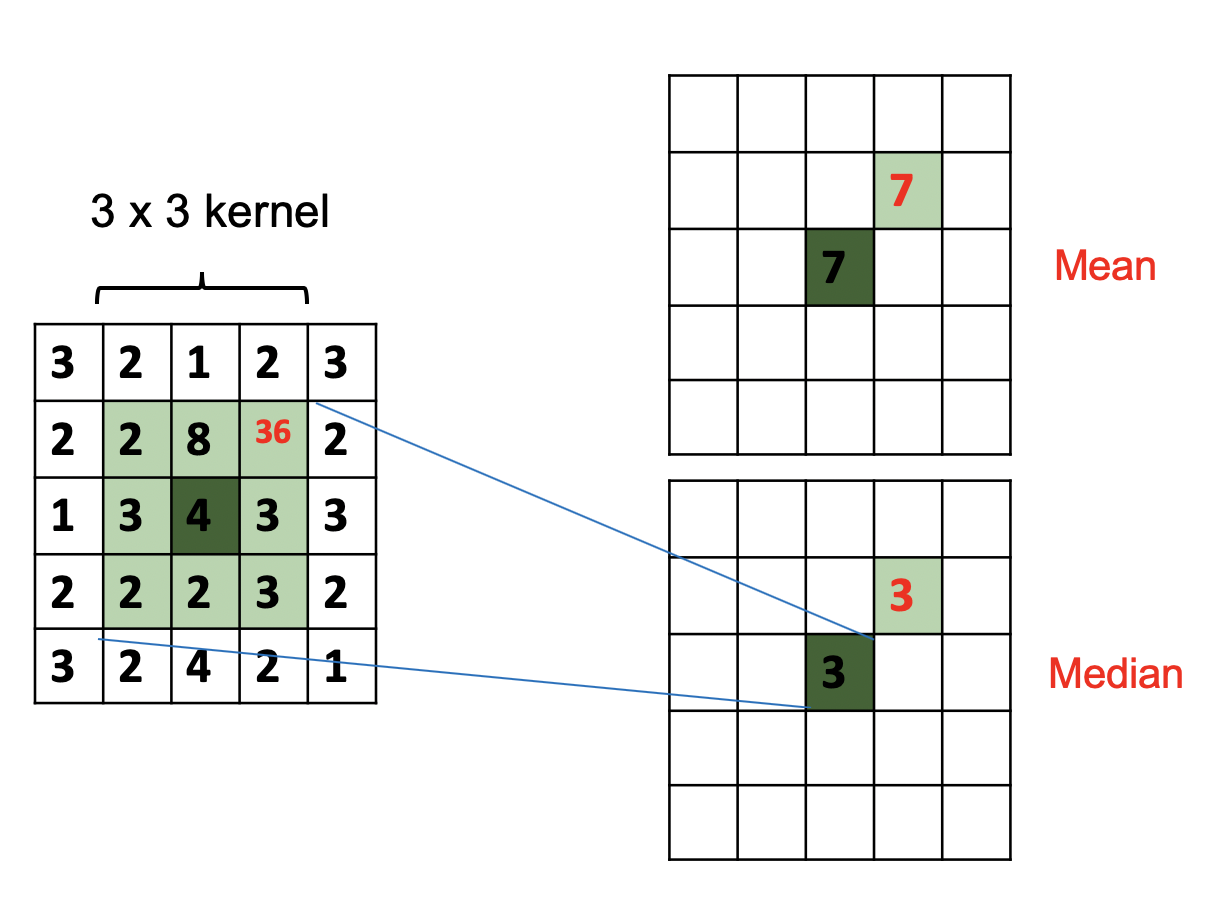
Mean Filter

clear; clf

% Load and display image
I = imread('coins.tif');
imshow(I)

% Apply a mean (or average) filter
H = fspecial('average', [3 3]); % H is our filter, we are creating a 3x3 mean filter
I_mean = imfilter(I, H); % apply the filter
imshow(I_mean)

Median Filter

I_median = medfilt2(I, [3 3]); % apply 3x3 median filter
imshowpair(I_mean, I_median, 'montage') % show images side-by-side

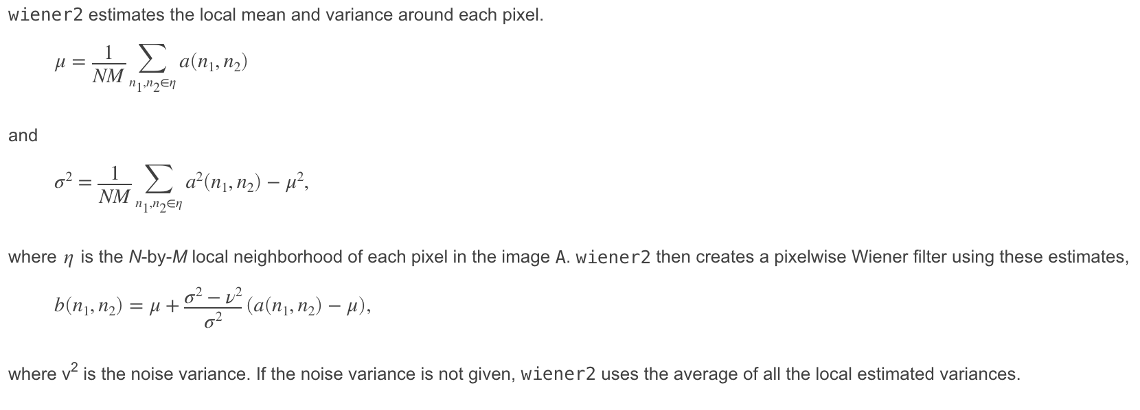
Example 4: Removing Gaussian Noise

clear; clf

% Load and display image
I = imread('planet.png');
imshow(I)

% Apply Wiener Filter
I_wiener = wiener2(I, [5 5]);

% Display the original and filtered images
imshowpair(I, I_wiener, 'montage')

Adjusting Image Contrast

Example 5: Adjusting Contrast Interactively

clear; clf

% Load the image
I = imread('colon_cells_1.tif');

% View the image in the Image Tool
imtool(I)

Using the Adjust Contrast Tool

Click the Adjust Contrast button in the toolbar (black and white circle).
Click and drag to change the bounds of the histogram.
Once satisfied with the contrast, click the “Adjust Data” button and close the Adjust Contrast Tool.
Export the new image to the workspace. File > Export to Workspace > Enter new variable name (Optional) > OK

Example 6: Automated Contrast Enhancement

imadjust saturates the bottom 1% and top 1% of pixels.

I_adj2 = imadjust(I);

imshowpair(I, I_adj2, 'montage')

Example 7: Batch Contrast Enhancement

clear; clf

% A for loop allows us to perform the same operation iteratively
for i = 1:6
    
    % Specify filename
    filename = strcat('colon_cells_', num2str(i), '.tif');
    
    % Load file
    I = imread(filename);

    % Adjust contrast
    I_adj = imadjust(I);
    
    % Save adjusted image as new file
    new_filename = strcat('a_', filename);
    imwrite(I_adj, new_filename)

end

Correcting Uneven Illumination

Example 8: Gaussian Blur and Image Math

clear; clf

% Load the image
I = imread('rice.png');

% Apply Gaussian blur to create background image
bg = imgaussfilt(I, 60);

% Show image and background
imshowpair(I, bg, 'montage')

% Subtract background from image
I_corr = I - bg;

% Show original and corrected images
imshowpair(I, I_corr, 'montage')

% Write out the corrected image (to be used later)
imwrite(I_corr, 'rice_corr.png')

Image Segmentation

Example 9: Detecting and Measuring Circular Objects

clear; clf

% Load the image
I = imread('colon_cells_1.tif');

% Adjust the contrast
I_adj = imadjust(I);

% Binarize the image
I_bw = imbinarize(I_adj);

% Determine radius range with imdistline tool
imshow(I_bw)
d = imdistline;
delete(d) % remove the imdistline tool

% Find circle centers and radii
[centers, radii] = imfindcircles(I_bw, [2 10], 'ObjectPolarity', 'bright');

% Display detected circles on image
imshow(I_adj)
h = viscircles(centers, radii);

% Try increasing sensitivity of circle detection
[centers, radii] = imfindcircles(I_bw, [2 10], 'ObjectPolarity', 'bright', 'Sensitivity', 0.9);

figure; % opens a new figure window
imshow(I_adj)
h = viscircles(centers, radii);

Example 10: Analyzing Foreground Objects

clear; clf

% Load the corrected rice image
I = imread('rice_corr.png');

% Adjust contrast
I_adj = imadjust(I);

% Binarize the image
I_bw = imbinarize(I_adj);

% Remove objects that are smaller than 50 pixels (not rice)
I_bw = bwareaopen(I_bw, 50);
imshow(I_bw)

% Fill in holes
I_bw = imfill(I_bw, 'holes');
imshow(I_bw)

% Identify objects (connected components) in the image
cc = bwconncomp(I_bw, 8);

% Extract areas of individual grains of rice
A = regionprops(cc, 'Area');

% Extract mean intensity values
meanInt = regionprops(cc, I, 'MeanIntensity');

Other properties in regionprops:

Area
Centroid
Major/Minor Axis Length
Perimeter
Max/Mean/Min Intensity

Image Registration

Example 11: Geometric Image Registration

clear; clf

% Load the images and convert to grayscale
im1 = rgb2gray(imread('arc-de-triomphe1.jpg'));
im2 = rgb2gray(imread('arc-de-triomphe2.jpg'));

% Display image differences
figure;
imshowpair(im1, im2, 'falsecolor')

% Detect features in both images
pts1 = detectSURFFeatures(im1);
pts2 = detectSURFFeatures(im2);

% Extract feature descriptors
[features1, validPts1] = extractFeatures(im1, pts1);
[features2, validPts2] = extractFeatures(im2, pts2);

% Match features using their descriptors
indexPairs = matchFeatures(features1, features2);

% Retrieve locations of matching points in each image
matched1 = validPts1(indexPairs(:,1));
matched2 = validPts2(indexPairs(:,2));

% Show point matches
figure;
showMatchedFeatures(im1, im2, matched1, matched2)

% Estimate the transformation that will move Image 2 to Image 1 space
[tform, inlier2, inlier1] = estimateGeometricTransform(matched2, matched1, 'similarity');

% Use the estimated transform to move Image 2 to Image 1 space
outputview = imref2d(size(im1)); % sets world coordinates given # of rows and columns
recovered = imwarp(im2, tform, 'OutputView', outputview);

figure;
imshowpair(im1, recovered, 'falsecolor')

Image Data Management with OMERO

With the advent of high-throughput screening, the need for efficient image management tools is greater than ever. From the microscope to publication, OMERO is a database solution that handles all your images in a secure central repository. You can view, organize, analyze and share your data from anywhere you have internet access. Work with your images from a desktop app (Windows, Mac or Linux), on UVA’s high performance computing platform (Rivanna), from the web, or through 3rd party software like Fiji and ImageJ, Python, and MATLAB. OMERO is able to read over 140 proprietary file formats, including all major microscope formats.

Example 12: Image Processing and Analysis with OMERO

%%%%%%%%%

% Sample MATLAB Image Processing pipeline with OMERO

%%%%%%%%%

%% Log into OMERO

myUsername = '';
myPassword = '';

    
%%%%% Don't change anything in this section! %%%%%
    
client = loadOmero('omero.hpc.virginia.edu',4064);
    
session = client.createSession(myUsername, myPassword);

%%%%%%%%%%%%%%%%%%%%%%%%%%%%%%%%%%%%%%%%%%%%%%%%%%%

%% Specify the Project and Dataset containing raw data

projectID = 107;

datasetID = 163;

%% Each image is processed and analyzed, then exported back to OMERO

%%%%% Don't change anything below this line! %%%%%

dataset = getDatasets(session, datasetID, true);
datasetName = char(dataset.getName().getValue());
imageList = dataset(1).linkedImageList;
imageList = imageList.toArray.cell;

newdataset = createDataset(session, 'binarized', ...
    getProjects(session,projectID));

for i = 1:length(imageList)
    pixels = imageList{i}.getPrimaryPixels();
    name = char(imageList{i}.getName().getValue());
    store = session.createRawPixelsStore();
    store.setPixelsId(pixels.getId().getValue(),false);
    plane = store.getPlane(0,0,0);
    img = uint8(toMatrix(plane,pixels));
    
    type = 'uint8';
    
    newimg = uint8(contrastIncrease(img));
    newimg = uint8(binarizeImage(newimg));
    newname = strcat('b_',name);
    
    pixelsService = session.getPixelsService();
    pixelTypes = toMatlabList(session.getTypesService().allEnumerations('omero.model.PixelsType'));
    pixelTypeValues = arrayfun(@(x) char(x.getValue().getValue()),pixelTypes,'Unif',false);
    pixelType = pixelTypes(strcmp(pixelTypeValues, type));
    
    description = sprintf('Dimensions: 512 x 512 x 1 x 1 x 1');
    
    idNew = pixelsService.createImage(512,512,1,1,toJavaList(0:0,'java.lang.Integer'),pixelType,newname,description);

    imageNew = getImages(session, idNew.getValue());
    
    link = omero.model.DatasetImageLinkI;
    link.setChild(omero.model.ImageI(idNew,false));
    link.setParent(omero.model.DatasetI(newdataset.getId().getValue(),false));
    session.getUpdateService().saveAndReturnObject(link);
    
    pixels = imageNew.getPrimaryPixels();
    store = session.createRawPixelsStore();
    store.setPixelsId(pixels.getId().getValue(),false);
    byteArray = toByteArray(newimg, pixels);
    
    store.setPlane(byteArray,0,0,0);
    store.save();
    store.close();
    
    cc = bwconncomp(newimg,4);
    numCells = num2str(cc.NumObjects);
    
    mapAnnotation = writeMapAnnotation(session,'Count',numCells);
    
    link = linkAnnotation(session, mapAnnotation, 'image', idNew.getValue());
end

client.closeSession();


function I3 = contrastIncrease(image)

    I = image;
    background = imopen(I,strel('disk',15));

    I2 = I - background;

    I3 = imadjust(I2);

end


function bw = binarizeImage(image)
    
    bw = imbinarize(image);
    bw = bwareaopen(bw, 10)*255;

end