MATLAB Data Processing and Visualization
MATLAB is mathematical computing software that combines an easy-to-use desktop environment with a powerful programming language. MATLAB can be used for data cleansing and processing, as well as data visualization. This tutorial will cover
- importing data from a variety of file types and formats, 2. data cleansing and manipulation, and 3. data visualization techniques.
Downloading the Data
Throughout the tutorial we will be working with data from the National Health and Nutrition Examination Survey (NHANES). Download nhanes_matlab.xlsx.
Data Import
Importing Tabular Data
readtable
Creates a table by reading column oriented data from a file
T = readtable(filename)
readtable creates one variable in the table T for each column in the file filename.
Wholly numeric columns will be converted to a numeric array; a cell array will be generated from a column containing any non-numeric values.
| Readable File Formats | File Extensions |
|---|---|
| Delimited text files | .txt, .dat, .csv |
| Spreadsheet files | .xls, .xlsb, .xlsx |
Example
data = readtable('nhanes_matlab.xlsx');
While readtable is capable of reading Excel files, you will need to use readmatrix if you
need to specify sheet names or a range of data. Both of these functions output a table.
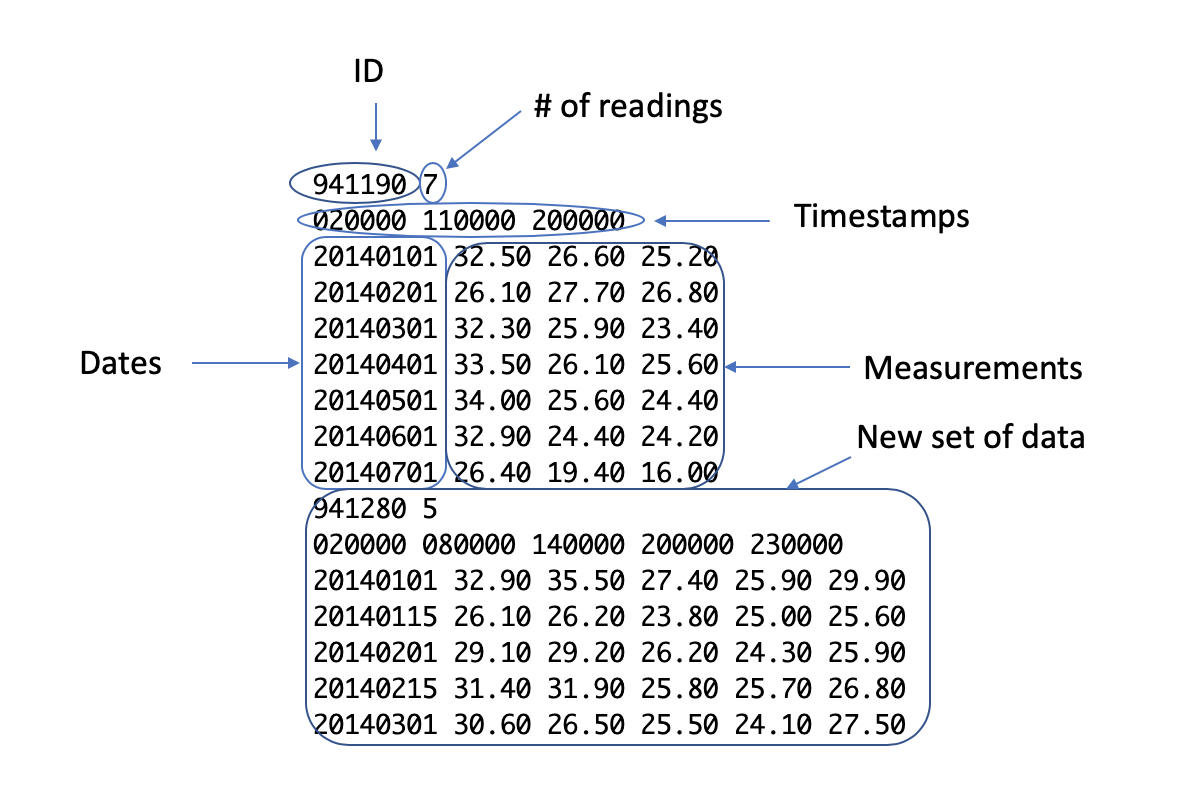
Importing Data from Multiple Files
datastore
Read large collections of data
A datastore is simply a reference to a file or set of files. You tell MATLAB where to look
for files with the datastore command.
Single File
ds = datastore(filename)
Multiple Files
ds = datastore(directory)
The datastore ds has many properties that you can modify so that MATLAB reads your data
correctly (e.g. treating -999 as a missing value instead of a numeric data point).
Datastores are also useful if you are working with such a large amount of data that you wouldn’t be able to load it all into memory. With a datastore you can tell MATLAB to read in the data incrementally, whether it’s file by file or in 100-line chunks (MATLAB reads data in 20,000 line chunks by default).
To read in data using a datastore, use the read or readall commands.
Read data incrementally
data = read(ds);
Read all data referenced by datastore ds
data = readall(ds);
See the MATLAB documentation on datastores to learn more about customizing your data import.
Example
% Create datastore
ds = datastore('nhanes_matlab.xlsx');

% Set ReadSize property in ds to 50 so we only read in 50 lines at a time
ds.ReadSize = 50;

% Read in first 50 lines
data50 = read(ds);

% Read in next 50 lines
data100 = read(ds);

% Read in all data
data_all = readall(ds);
Importing Unstructured Data
Suppose you have an unstructured data file like the one below.
MATLAB is unable to read data automatically if each line doesn’t have the same number of columns. We can use MATLAB’s lower-level file import functions to read irregular data.
Using low-level file import requires three steps:
-
Open file (
fid = fopen(filename), fid stands for file ID) -
Read data
-
Close file (
fclose(fid))
The first and last steps are pretty straightforward, so the rest of this section will focus on step 2. There are a couple ways we can read in the data.
fgetl
Read line from file
myLine = fgetl(fid)
Using in succession will allow you to continue reading the file line by line. Regardless of
whether the data is numeric, the output of fgetl will be a string. This means you may have to
parse and convert the data to the proper data type after import. You can learn more about
this process from
MATLAB’s documentation on string manipulation.
textscan
Read formatted data from file
myData = textscan(fid, formatSpec)
textscan allows you to specify the format of a line of data up-front so that you don’t have to
manipulate strings unnecessarily. textscan also allows you to read multiple lines and to skip
any columns you don’t need.
The output of textscan is a cell array (myData) where each cell contains the values from a
single column. Each cell will contain a column vector (for numeric data) or column cell array (for non-numeric or mixed
data).
textscan requires you to specify the format of your data in the variable formatSpec.
Below is a formatSpec for some example data.
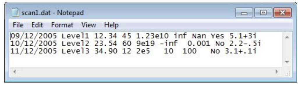
% This dataset is part of your installation of MATLAB!

% fullfile retrieves the full file path to the dataset.
filename = fullfile(matlabroot, 'examples', 'matlab', 'scan1.dat');

% Open the file
fid = fopen(filename);

% Format spec: it's a string
formatSpec = '%{MM/dd/uuuu}D %s %f32 %d8 %u %f %f %s %f';

% Read the data into using textscan
myData = textscan(fid, formatSpec);

% Close the file
fclose(fid);
More information about MATLAB’s low-level file I/O can be found here: https://www.mathworks.com/help/matlab/low-level-file-i-o.html.
Data Cleansing
Working with Missing Data
When MATLAB imports data that has missing values for numeric variables, it replaces that
instance with NaN, or Not-a-Number. This section discusses multiple ways you
can handle missing data and NaNs.
Omitting NaNs
Calculating statistics on arrays that contain NaN results in another NaN. If we want to omit NaNs
from our calculation, we can use the 'omitnan' option.
Example: Calculating mean
avgIncome = mean(data.Income, 'omitnan');
Other functions that can use the 'omitnan' option:
| Function Name | What It Does |
|---|---|
| cov | Covariance |
| mean | Mean |
| median | Median |
| std | Standard Deviation |
| var | Variance |
However, max and min omit NaNs by default, and adding the 'omitnan' flag will yield
unexpected results.
Locating Missing Data and Deleting Incomplete Rows
ismissing
Find missing values in a table
TF = ismissing(A)
ismissing returns a logical array TF that is the same size as the table A. Values of 1
in TF correspond to missing values in A at the same location.
any
Find non-zero elements in an array
missingRows = any(TF, 2)
any returns a logical array missingRows that is the same length as the input array TF.
Values of 1 in missingRows correspond to rows in TF that contain a 1. Because 1s in TF
correspond to missing values in our original table A, values of 1 in missingRows also correspond
to rows with missing data in A.
We have the number 2 as the second input in any. This is because by default any looks for
non-zero elements in a column. Since we want to look for non-zero elements in rows, we need to specify
that with the 2.
Logical Indexing
Remove rows with missing data
A(missingRows,:) = [];
Using our logical array missingRows, we can index into our table A and select all the
rows in A that have missing data. With the colon operator :, we can also select the data from all
the columns in those rows. If we select that data in A and set it equal to empty brackets, that will
remove all those rows from A.
Example
% Read in data as table
data = readtable('nhanes_matlab.xlsx');

% Find missing data
missing = ismissing(data);

% Find rows that have missing data
missingRows = any(missing, 2);

% Remove rows with missing data from table
data(missingRows,:) = [];
Categorical Data and Set Operations
categorical
Assigns a value to each of a finite set of discrete categories
Consider the cell array below.
mySet = {'low', 'medium', 'low', 'low', 'high', 'medium', 'low'};
As humans, we understand that the array contains values that fall into 3 distinct categories:
‘low’, ‘medium’, and ‘high’. MATLAB doesn’t necessarily know this and will treat all seven items in the
array as individual values. With the categorical function, we can tell MATLAB to treat values with
the same string as part of a single category. The output of the categorical function is a
categorical array the same size as the input array.
mySet = categorical(mySet);

categories(mySet)
With the categories command, we can find out the different categories in our categorical array.
As expected, our three categories are ‘low’, ‘medium’, and ‘high’.
We can convert the text variables in our table to categorical arrays one at a time with the categorical command.
% Reading the data into a table
data = readtable('nhanes_matlab.xlsx');

% Convert Gender variable to categorical array
data.Gender = categorical(data.Gender);
convertvars
Batch convert table variables to categorical arrays
T2 = convertvars(T1, vars, datatype)
We can use convertvars to create a new table T2 that converts all the variables in our table T1 to our desired data
type, in this case categorical arrays. We list the names of the variables we want to convert in
the cell array vars.
Example
% Reading the data into a table
data = readtable('nhanes_matlab.xlsx');

% Convert text variables to categorical arrays
vars = {'Gender', 'Race'};

newdata = convertvars(data, vars, 'categorical');
We can replace vars with @iscell if we know we want to convert all cell arrays to in our
table to categorical arrays.
newdata = convertvars(data, @iscell, 'categorical');
Why Use Categorical Arrays?
- Several discrete data plot types require input data be categorical
- Use less memory
ismissingis able to determine missing data in categorical arrays but not cell arrays
Analyzing Groups within Data
Data Visualization
We will be looking at different examples of data visualization in MATLAB using a live script. Please download the script from this link.
plot and Modifying Plot Line Properties
Functions for Customizing Appearance
-
Figure Formatting GUI
-
Exporting and Saving Figures
-
Log-Scaled Axes
-
Bar Plots, Box Plots, and Histograms
-
Scatter Plots
-
Scatter Plot Matrix
-
3-D Surface Plots
-
Animation
Extra Exercises
NHANES
-
Create a scatter plot of Height vs Weight. Include labels on both axes and a title for your graph.
-
Create a new table in which all rows containing missing data, categorical or numerical, have been removed.
-
Create a scatter plot matrix to compare Weight, Height, and BPSys.
-
Create stacked bar plots showing the proportions of the Highest Level of Education reached at each Income.