Parallel/GPU Computing
Why go parallel?
- Speed - Solve a problem more quickly
- Scale - Solve a larger, more complex problem with higher fidelity
- Throughput - Solve many (simple) problems more quickly
Parallel Computing Myths
Myth #1: Throwing more hardware at a problem will automatically reduce the time to solution.
Parallel computing will only help if you have an application that has been written to take advantage of parallel hardware. And even if you do have a parallel code, there is an inherent limit on scalability. (Caveat - a high-throughput computing workload can use parallel computing to run many single-core/GPU instances of an application to achieve near perfect scaling.)
Myth #2: You need to be a programmer or software developer to make use of parallel computing.
Most users of parallel computers are not programmers. Instead, they use mature third-party software that had been developed elsewhere and made available to the community.

Processes and Threads
Threads and processes are both independent sequences of execution.
- Process: instance of a program, with access to its own memory, state, and file descriptors (can open and close files)
- Incur more overhead
- Are more flexible - multiple processes can be run within a compute node or across multiple compute nodes (distributed memory)
- Thread: lightweight entity that executes inside a process. Every process has at least one thread, and threads within a process can access shared memory.
- Incur less overhead
- Threaded codes can use less memory since threads within a process have access to the same data structures
- Are less flexible - multiple threads associated with a process can only be run within a compute node (shared memory)
Online resources describing the differences between thread and processes tend to be geared towards computer scientists, but the following resources do a reasonable job of addressing the topic:
- https://stackoverflow.com/questions/200469/what-is-the-difference-between-a-process-and-a-thread (more technical)
- https://www.educba.com/process-vs-thread/ (more informal)
The Importance of Processes and Threads
The type of parallelization will determine how and where you will run your code.
- Distributed-memory applications (multiple processes/instances of a program) can be run on one or more nodes.
- Shared-memory (threaded) applications should be run on a single node.
- Hybrid applications can be run on one or more nodes, but you should consider the balance between threads and processes (discussed later).
- In all cases, you may need to consider how processes and threads are mapped and bound to cores.
In addition, being aware of threads and processes will help you to understand how your code is utilizing the hardware and identify common problems.
Message Passing Interface
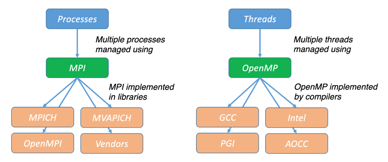
MPI is a standard for parallelizing C, C++, and Fortran code to run on distributed memory (multiple compute node) systems. While not officially adopted by any major standard bodies, it has become the de facto standard (i.e., almost everyone uses it).
There are multiple open-source implementations, including OpenMPI, MVAPICH, and MPICH along with vendor-supported versions. MPI applications can be run within a shared-memory node. All widely-used MPI implementations are optimized to take advantage of the faster intranode communications. MPI is portable and can be used anywhere. Although MPI is often synonymous with distributed memory parallelization, other options are gaining adoption (Charm++, UPC, X10).
OpenMP
OpenMP is an application programming interface (API) for shared-memory (within a node) parallel programming in C, C++, and Fortran.
OpenMP provides a collection of compiler directives, library routines, and environment variables. OpenMP is supported by all major compilers, including IBM, Intel, GCC, PGI, and AMD Optimizing C/C++ Compiler (AOCC). OpenMP is portable and can be used anywhere. Although OpenMP is often synonymous with shared-memory parallelization, there are other options: Cilk, POSIX threads (pthreads) and specialized libraries for Python, R, and other programming languages.
Amdahl’s Law and Limits on Scalability
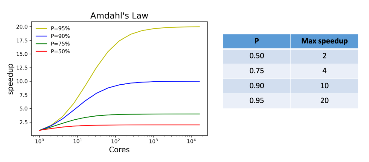
Amdahl’s law describes the absolute limit on the speedup of a code as a function of the proportion of the code that can be parallelized and the number of processors. This is the most fundamental law of parallel computing!
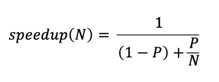
P is the fraction of the code that can be parallelized, S is the fraction of the code that must be run sequentially (S=1-P), and N is the number of processors.
In the limit as the number of processors goes to infinity, the theoretical speedup depends only on the proportion of the parallel content.
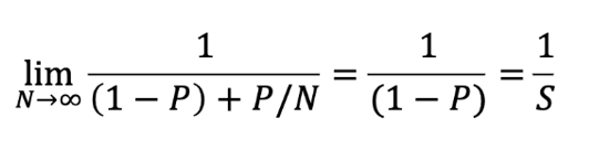
That doesn’t look so bad, but as you’ll see next, it doesn’t take much serial content to quickly impact the speedup.
Other Limits on Scalability
Amdahl’s law sets a theoretical upper limit on speedup, but there are other factors that affect scalability:
- Communications overhead
- Problem size
- Uneven load balancing
In real-life applications that involve communications, synchronization (all threads or processes must complete their work before proceeding), or irregular problems (non-cartesian grids), the speedup can be much less than predicted by Amdahl’s law.
Running Parallel Applications
So far, we’ve covered the basic concepts of parallel computing – hardware, threads, processes, hybrid applications, implementing parallelization (MPI and OpenMP), Amdahl’s law, and other factors that affect scalability.
Theory and background are great, but how do we know how many CPU’s GPUs to use when running our parallel application? The only way to definitively answer this question is to perform a scaling study where a representative problem is run on different number of processors. A representative problem is one with the same size (grid dimensions; number of particles, images, genomes, etc.) and complexity (e.g., level of theory, type of analysis, physics, etc.) as the research problems you want to solve.
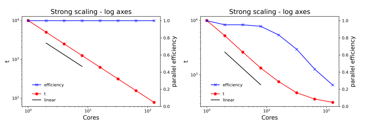
Presenting Scaling Results
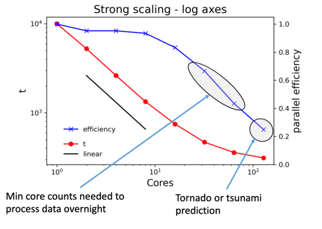
Plotting the same data on log axes gives a lot more insight. Note the different scales for the left axes on the two plots. Including a line showing linear scale and plotting the parallel efficiency on the right axis adds even more value.
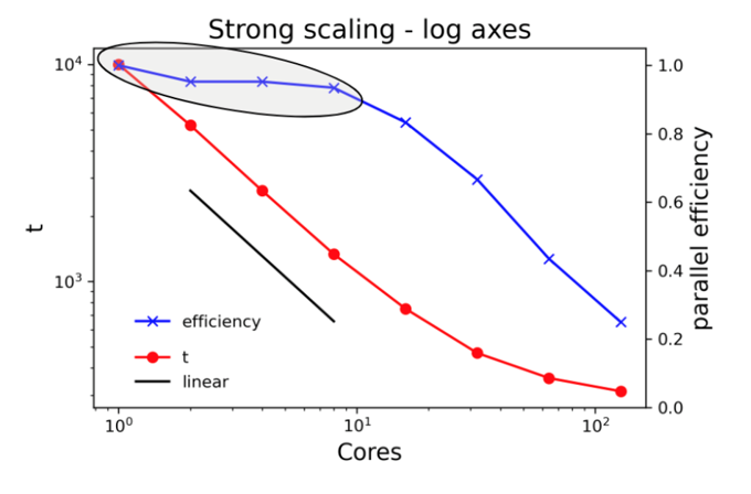
Where should I be on the scaling curve?
If your work is not particularly sensitive to the time to complete a single run, consider using a CPU/GPU count at or very close to 100% efficiency, even if that means running on a single core. This especially makes sense for parameter sweep workloads where the same calculation is run many times with different sets of inputs.
Go a little further out on the scaling curve if the job would take an unreasonably long time at lower core counts or if a shorter time to solution helps you make progress in your research. If the code does not have checkpoint-restart capabilities and the run time would exceed queue limits, you’ll have no choice but to run at higher core counts.
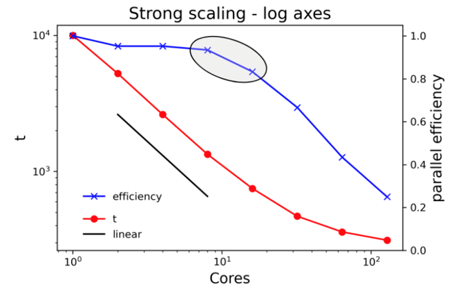
If the time to solution is absolutely critical, it’s okay to run at lower efficiency. Examples might include calculations that need to run on a regular schedule (data collected during day must be processed overnight) or severe weather forecasting.
Parallel Computing Summary
- Parallel computing is for everyone who wants to accomplish more research and solve more challenging problems
- You don’t need to be a programmer, but you do need to know some of the fundamentals to effectively use parallel computers
- Processes are instances of programs; threads run within a process and access shared data; MPI and OpenMP are used to parallelize codes
- Amdahl’s law imposes an upper limit on scalability, but there are other factors that impact scalability (load imbalance, communications overhead)
- Know how to display your scaling data and choose core counts
For code used to generate some figures in these notes, see https://github.com/sinkovit/Parallel-concepts
GPU vs CPU Architecture
CPU:
- Few processing cores with sophisticated hardware
- Multi-level caching
- Prefetching
- Branch prediction
GPU:
- Thousands of simplistic compute cores (packaged into a few multiprocessors)
- Operate in lock-step
- Vectorized loads/stores to memory
- Need to manage memory hierarchy
GPU Accelerated Software
Examples can be found from virtually any field:
- Chemistry
- Life sciences
- Bioinformatics
- Astrophysics
- Finance
- Medical imaging
- Natural language processing
- Social sciences
- Weather and climate
- Computational fluid dynamics
- Machine learning
Exhaustive list of software can be found here: https://www.nvidia.com/en-us/data-center/gpu-accelerated-applications/
GPU Accelerated Libraries
Ease of use:
- GPU acceleration without in-depth knowledge of GPU programming “Drop-in”
- Many GPU accelerated libraries follow standard APIs
- Minimal code changes required Quality
- High-quality implementations of functions encountered in a broad range of applications Performance
- Libraries are tuned by experts
Use libraries if you can - do not write your own matrix multiplication.
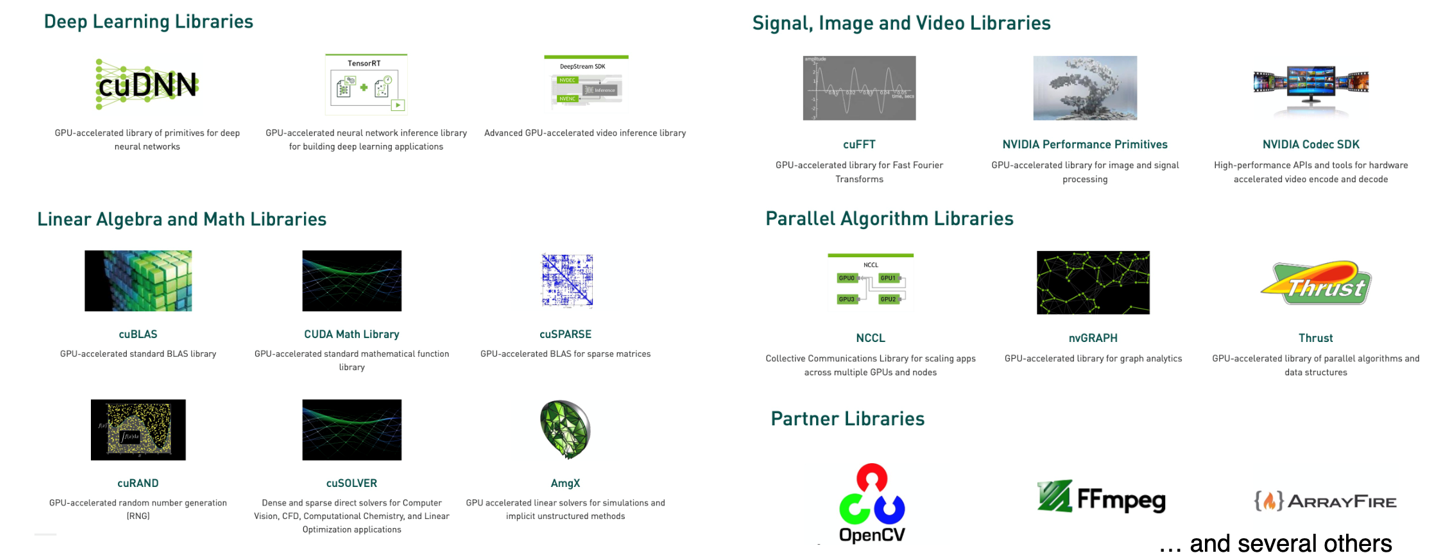
See https://developer.nvidia.com/gpu-accelerated-libraries for more info.
Numerical Computing in Python

NumPy:
- Mathematical focus
- Operates on arrays of data
- ndarray, holds data of same type
- Many years of development
- Highly tuned for CPUs
CuPy:
- NumPy-like interface
- Trivially port code to GPU
- Copy data to GPU
- CuPy ndarray
- Data interoperability with DL frameworks, RAPIDS, and Numba
- Uses high tuned NVIDIA libraries
- Can write custom CUDA functions
CuPy: a NumPy like interface to GPU-acceleration ND-Array operations
Before (with NumPy):
import numpy as np

size = 4096
A = np.random.randn(size,size)

Q, R = np.lingalg.qr(A)
After (with CuPy):
import cupy as np

size = 4096
A = np.random.randn(size,size)

Q, R = np.lingalg.qr(A)

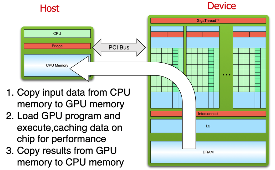
Processing Flow