Benchmarking Parallel Programs

Oct 29, 2020

Motivation

True or false:

“If I use more cores/GPUs, my job will run faster.”
“I can save SU by using more cores/GPUs, since my job will run faster.”
“I should request all cores/GPUs on a node.”

Show answer

1. Not guaranteed.
2. False!
3. Depends.

New HPC users may implicitly assume that these statements are true and request resources that are not well utilized. The disadvantages are:

Wasted SU. All requested cores/GPUs count toward the SU charge, even if they are idle. (SU is the “currency” for resource usage on a cluster. The exact definition will be presented later.)
Long waiting time. The more resources you request, the longer it is likely to wait in the queue.
Unpleasant surprise to see little or no performance improvement.

The premise of parallel scalability is that the program has to be parallelizable. Please read the documentation of your program to determine whether there is any benefit of using multiple cores/GPUs. (Exception: A serial program may need more memory than a single core can provide. You will need to request multiple cores, but this is a memory-bound issue and is different from the execution speed. We shall not consider this scenario for the remainder of the tutorial.)

What is benchmarking? And why/when should I benchmark?

A benchmark is a measurement of performance. We will focus on the execution time of a program for a given task. (This is also known as strong scaling in parallel computing.) However, even for a serial program, a benchmark can still be useful when you run the program on different platforms. For instance, if a certain task takes 1 hour to complete on your laptop and 5 hours on Rivanna, there could be something wrong with how the program was installed on Rivanna.

But doesn’t benchmarking cost SU? Two things. First, the dev partition is the perfect choice for benchmarking and debugging purposes, as long as you stay within the limits. Remember, you do not need to complete the entire task if it takes too long; a fixed subtask would do. This could be an epoch in machine learning training, a time step in molecular dynamics simulation, a single iteration, etc., instead of reaching full convergence. This way you can perform the benchmark without spending SU.

Second, if the benchmark cannot be performed on dev for whatever reason (e.g. even the smallest subtask would take more than 1 hour, or the job needs more cores than the limit), it is true that you will have to spend SU for benchmarking, but you may still gain in the long term, especially if you are running many production jobs of a similar nature (high-throughput). If you manage to prevent overspending say 10 SU per job, then after 10,000 jobs you would have saved 100k SU, an entire allocation. (Linear term trumps constant, eventually.)

Besides the amount of hardware, sometimes certain parameters of a program can have a huge impact on performance as well (e.g. batch size in machine learning training, NPAR/KPAR in VASP). You will need to find the optimum parameter to achieve the best performance specific to your problem. This may not translate across platforms - what’s optimal on one platform can be suboptimal on another, so you must perform a benchmark whenever you use a different platform!

Benchmarking will also help you get a better sense of the scale of your project and how many SU it entails. Instead of blindly guessing, you will be able to request cores/GPUs/walltime wisely.

Concepts and Theory

Definitions

Denote the number of cores (or GPU devices) as $N$ and the walltime as $t$. The reference for comparison is the job that uses $N=1$ and has a walltime of $t_1$.

Speedup is defined as $s=t_1/t$. For example, a job that finishes in half the time has a speedup factor of 2.

Perfect scaling is achieved when $N=s$. If you manage to halve the time ($s=2$) by doubling the resources ($N=2$), you achieve perfect scaling.

On Rivanna, the SU (service unit) charge rate is defined as $$SU = (N_{\mathrm{core}} + 2N_{\mathrm{gpu}}) t,$$ where $t$ is in units of hours.

We can define a relative SU, i.e. the SU relative to that of the reference: $$\frac{SU}{SU_1} = \frac{Nt}{t_1} = \frac{N}{s}.$$

In the case of perfect scaling, $N=s$ and so the relative SU is 1, which means you spend the same amount of SU for the parallel job as for its serial reference. Since sublinear scaling ($s<N$) almost always occurs, the implication is that you need to pay an extra price for parallelization. For example, if you use 2 cores ($N=2$) and reduce the walltime by only one-third ($s=1.5$), then the relative SU is equal to $N/s=1.33$, which means you spend 33% more SU than the serial job reference. Whether this is worth it will of course depend on:

the actual value of $s$,
the maximum walltime limit for the partition on Rivanna, and
your deadline.

Amdahl’s Law

A portion of a program is called parallel if it can be parallelized. Otherwise it is said to be serial. In this simple model, a program is strictly divided into parallel and serial portions. Denote the parallel portion as $p$ ($0 \le p \le 1$) and the serial portion as $1-p$ (so that the sum equals 1).

Suppose the program takes a total execution time of $t_1$ to run completely in serial. Then the execution time of the parallelized program can be expressed as a function of $N$: $$t = \left[(1-p) + \frac{p}{N}\right] t_1,$$ where the time spent in the serial portion, $(1-p)t_1$, is irrespective of $N$.

The speedup is thus $$s=\frac{t_1}{t} = \frac{1}{1-p+\frac{p}{N}}.$$

As $N\rightarrow\infty$, $s\rightarrow 1/(1-p)$. This is the theoretical speedup limit.

Exercise: a) Find the maximum speedup if 99%, 90%, 50%, 10%, and 0% of the program is parallelizable. b) For $N=100$, what is the relative SU in each case?

Show answer

a) 100, 10, 2, 1.11, 1.

b) First calculate the actual speedup (not the theoretical limit): 50.25, 9.17, 1.98, 1.11, 1.
Relative SU: 1.99, 10.9, 50.5, 90.1, 100.

Notice how the wasted SU increases dramatically.

Exercise: What is the theoretical limit in relative SU? $$\lim_{N\rightarrow\infty} \frac{SU}{SU_1}$$ Hint: Consider cases $s<N$ and $s=N$ separately.

Show answer

For perfect scaling, the relative SU is equal to 1 for all values of N.
Otherwise, no limit/undefined/goes to infinity.

Tools

The performance is usually tracked by the execution time.

`time`

The time command is included in most Linux distributions. You can simply prepend it to whatever command you want to time. For example:

$ time sleep 5

real    0m5.026s
user    0m0.001s
sys     0m0.006s

Notice there are 3 lines of output - real, user, and sys. A good explanation of these can be found here; for this tutorial, it is sufficient to use the real time. (The CPU time is given by user + sys, which in this case is almost 0 because the command is just sleep.)

`perf`

A more dedicated tool for performance measurement is perf. Instead of a single measurement, it is more accurate to run a benchmark multiple times and take the average. The perf tool contains built-in statistical analysis. Advanced users please refer to the official tutorial. Load the module if you would like to use perf: module load perf.

If you just want to get a rough idea with an error bar of say 5-10%, time suffices. The task should last significantly longer than 1 second.

Examples

Multi-core: Gaussian

Gaussian is a quantum chemistry software package that can run on multiple CPU cores. This example is the open-shell vanilomycin test (#0709) included with the software.

Setup

First load the module:

module load gaussian

If you are using Gaussian only through a course:

module load gaussian/grads16

Copy the input file:

cp $g16root/g16/tests/com/test0709.com .

Prepare a SLURM script (job.slurm):

#!/bin/bash
#SBATCH -A <my_allocation>
#SBATCH -p standard
#SBATCH -t 10:00:00
#SBATCH -N 1
#SBATCH -c 1
#SBATCH -C skylake

module purge
module load gaussian  # or gaussian/grads16
hostname
grep -c processor /proc/cpuinfo
cp $g16root/g16/tests/com/test0709.com .
g16 -p=$SLURM_CPUS_PER_TASK test0709.com

Note:

The number of cores (#SBATCH -c <num>) is passed through the $SLURM_CPUS_PER_TASK environment variable to Gaussian’s -p flag. This ensures consistency.
$g16root is an environment variable made available to you after you load the Gaussian module.
The time command is not needed here because Gaussian will time the job automatically.

Submit the job:

sbatch job.slurm

Benchmark

Modify the SLURM script to use 4, 8, 16, and 32 cores. Submit these jobs. The walltime can be read from the test0709.log file.

$ grep Elapsed test0709.log
 Elapsed time:       0 days  0 hours 15 minutes 35.4 seconds.

You should obtain similar results as follows:

N	Time (s)	Speedup	Relative SU
1	12323.9	1.00	1.00
4	2968.3	4.15	0.96
8	1528.5	8.06	0.99
16	935.4	13.18	1.21
32	842.2	14.63	2.19

Don’t get excited about the apparent superlinear scaling ($s>N$ for $N=4,8$) - it is within the margin of error.

The speedup is plotted below. Notice the perfect scaling up to $N=8$. The scaling performance worsens beyond 8 cores and drastically beyond 16. This does not mean 8 is the magic number to use for all Gaussian jobs - it only applies to calculations of a similar nature.

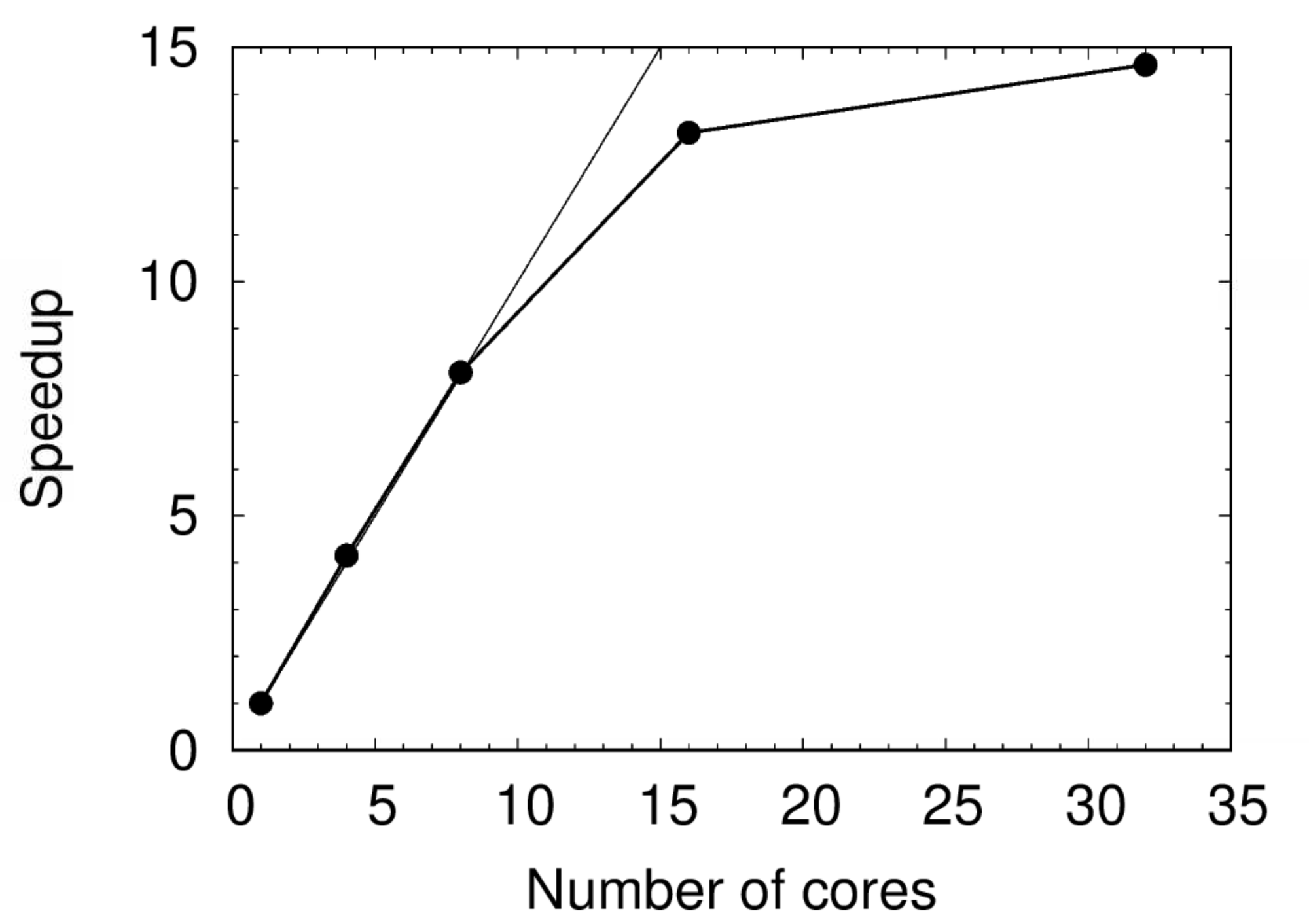
Exercise: Does this obey Amdahl’s Law? Why or why not?

Multi-GPU: PyTorch

PyTorch can make use of multiple GPU devices through the DistributedDataParallel (DDP) backend. This example is based on our PyTorch 1.7 container using the Python script provided by PyTorch Lightning with minor modifications. (The container uses CUDA 11 which is compatible with Rivanna hardware after the December 2020 maintenance.)

Setup

Download the container. The following command will create a Singularity container pytorch_1.7.0.sif.

module load singularity
singularity pull docker://uvarc/pytorch:1.7.0

Copy the following as a plain text file (example.py).

import os
import torch
from torch import nn
import torch.nn.functional as F
from torchvision.datasets import MNIST
from torch.utils.data import DataLoader, random_split
from torchvision import transforms
import pytorch_lightning as pl

class LitAutoEncoder(pl.LightningModule):

    def __init__(self):
        super().__init__()
        self.encoder = nn.Sequential(nn.Linear(28 * 28, 128), nn.ReLU(), nn.Linear(128, 3))
        self.decoder = nn.Sequential(nn.Linear(3, 128), nn.ReLU(), nn.Linear(128, 28 * 28))

    def forward(self, x):
        # in lightning, forward defines the prediction/inference actions
        embedding = self.encoder(x)
        return embedding

    def training_step(self, batch, batch_idx):
        # training_step defined the train loop. It is independent of forward
        x, y = batch
        x = x.view(x.size(0), -1)
        z = self.encoder(x)
        x_hat = self.decoder(z)
        loss = F.mse_loss(x_hat, x)
        self.log('train_loss', loss)
        return loss

    def validation_step(self, batch, batch_idx):
        x, y = batch
        x = x.view(x.size(0), -1)
        z = self.encoder(x)
        x_hat = self.decoder(z)
        loss = F.mse_loss(x_hat, x)
        self.log('val_loss', loss)
        return loss

    def configure_optimizers(self):
        optimizer = torch.optim.Adam(self.parameters(), lr=1e-3)
        return optimizer

dataset = MNIST(os.getcwd(), download=True, transform=transforms.ToTensor())
train, val = random_split(dataset, [55000, 5000])

autoencoder = LitAutoEncoder()
trainer = pl.Trainer(max_epochs=1, gpus=1)
trainer.fit(autoencoder, DataLoader(train), DataLoader(val))

Prepare a SLURM script (job.slurm) that runs the above Python script. We would like to download the MNIST data files first and exclude the download time from the actual benchmark. (More on this later.) Also specify a GPU type for consistency.

#!/bin/bash
#SBATCH -A <myallocation>
#SBATCH -t 00:10:00
#SBATCH -N 1
#SBATCH --ntasks-per-node=1
#SBATCH -p gpu
#SBATCH --gres=gpu:1

module purge
module load singularity

time singularity run --nv pytorch_1.7.0.sif example.py

Submit the job.

sbatch job.slurm

Benchmark

Set download=False in example.py:

dataset = MNIST(os.getcwd(), download=False, transform=transforms.ToTensor())

Resubmit the job to set the reference ($t_1$). Next, to make use of multiple GPU devices, use the ddp backend:

trainer = pl.Trainer(max_epochs=1, gpus=2, distributed_backend='ddp')

For this example, use the same number in --ntasks-per-node and --gres=gpu in your SLURM script. Also add srun (important):

time srun singularity run --nv pytorch_1.7.0.sif example.py

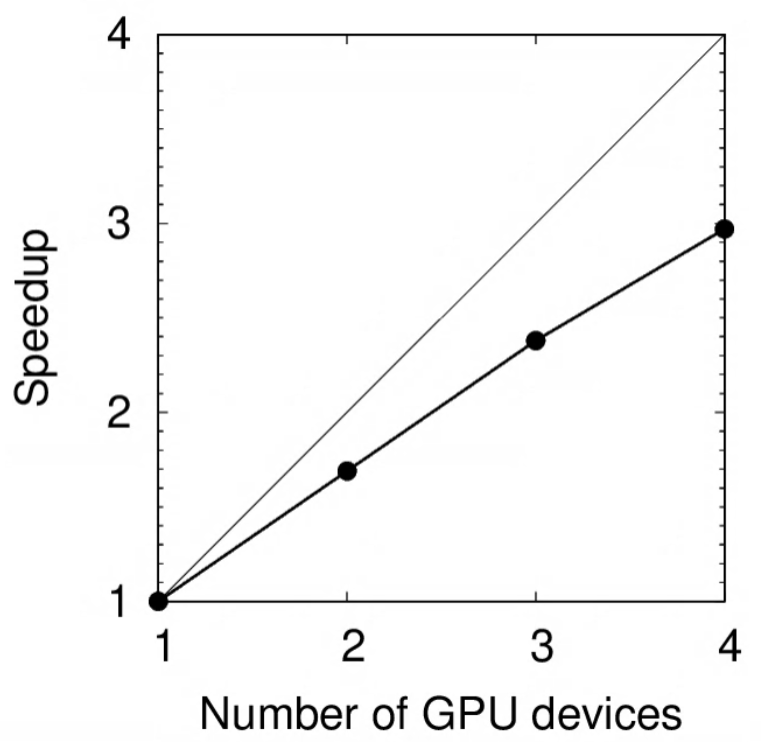
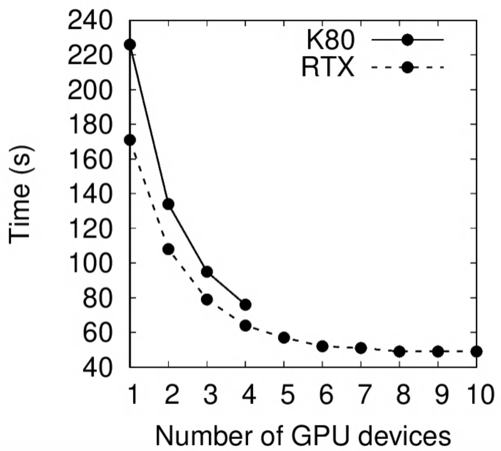
Results on a K80 GPU:

N	Time (s)	Speedup	Relative SU
1	226	1.00	1.00
2	134	1.69	1.18
3	95	2.38	1.26
4	76	2.97	1.35

The speedup is plotted below. Notice how the deviation from perfect scaling (light diagonal line) increases with $N$.

The same benchmark was performed on RTX 2080Ti:

N	Time (s)	Speedup	Relative SU
1	171	1.00	1.00
2	108	1.58	1.26
3	79	2.16	1.39
4	64	2.67	1.50
5	57	3.00	1.67
6	52	3.29	1.82
7	51	3.35	2.09
8	49	3.49	2.29
9	49	3.49	2.58
10	49	3.49	2.87

Notice the plateau beyond $N=6$, which implies that you should not request more than 6 GPU devices for this particular task. (A good balance between speed and SU effectiveness may be $2\le N \le 4$.)

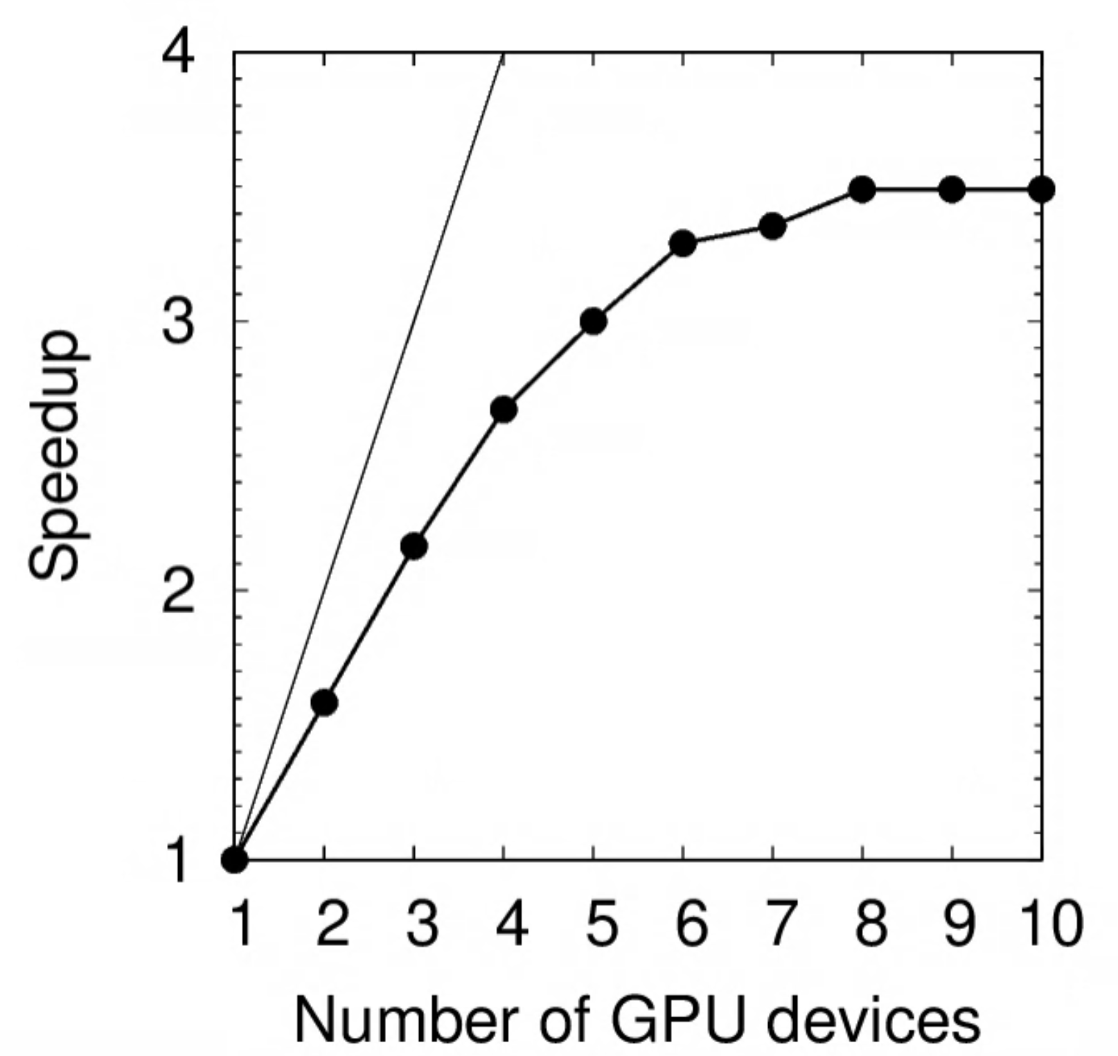
Exercise: Deduce the parallel portion $p$ of this program using Amdahl’s Law.

Show answer

Using $s=3.49$ as the theoretical speedup limit, $p=1-1/s=0.71$.

The performance of K80 vs RTX 2080Ti is compared below. On a single GPU device, the latter is 30% faster.

Remarks

A complete machine learning benchmark would involve such parameters as batch size, learning rate, etc. You may pass a sparse grid to locate a desirable region and, if necessary, use a finer grid in that region to identify the best choice.

Exercise: Revisit the true-or-false questions at the beginning of this tutorial and answer them in your own words.

Exercise: A user performed a benchmark on the standard partition and determined that a serial job would take 10 days to complete and that the theoretical speedup limit is 4. The entire project involves 1,000 such jobs. Assume that all 1,000 jobs can start running immediately. (The standard partition has a walltime limit of 7 days. No job extensions can be granted.)
a) What is the minimum amount of SU needed to finish the entire project?
b) The user has a deadline of 3 days. How many cores should the user request per job? How many extra SU will need to be spent compared to the minimum in a)?
c) Suppose the user did not perform the benchmark and just randomly decided to use 20 cores per job. How much time and how many SU will the user spend for this project? Compare your answer with b).
d) Repeat b) but this time the deadline is in 50 hours.

Show answer

a) Since each job could not finish within the 7-day limit using 1 core, we need to find the smallest $N$ such that $t\le7$ days. On one hand, the restriction is $$s=\frac{t_1}{t}\ge \frac{10}{7};$$ on the other hand, we know $s_{\max}=1/(1-p) = 4$ so $p=0.75$ and that $$s= \frac{1}{0.25+\frac{0.75}{N}}.$$ Combining these two equations: $$\frac{1}{0.25 +\frac{0.75}{N}} \ge \frac{10}{7}$$ $$0.25+\frac{0.75}{N} \le \frac{7}{10}$$ $$N \ge \frac{0.75}{0.7-0.25} \approx 1.67.$$ Since $N$ must be an integer, the smallest solution is 2. For $N=2$, we obtain $$s= \frac{1}{0.25+\frac{0.75}{2}} = 1.6$$ and $$t= t_1/s = 10\times24/1.6 = 150\ \mathrm{hours}$$ or 6 days and 6 hours. Hence, each job takes $Nt=2\times 150=300$ SU and the entire project needs 300k SU.

b) Using the derivation in a) we find $$N \ge \frac{0.75}{\frac{3}{10}-0.25} = 15.$$ The total amount of SU is $$15\times(3\times24)\times 1000 = 1.08\mathrm{M}.$$ Compared to the minimum, the user needs to spend an extra 780k SU.

c) For $N=20$ we obtain $$s= \frac{1}{0.25+\frac{0.75}{20}} \approx 3.48$$ and $$t = 10\times24/3.48 = 69\ \mathrm{hours}$$ or 2 days and 21 hours. Each job costs $20\times69=1.38$k SU and the entire project needs 1.38M SU. Compared to b) the project takes 3 hours less but at an additional cost of 300k SU.

d) Unfortunately, the user will not be able to meet the deadline, since even with an infinite amount of cores each job would take $10\times24/4=60$ hours.

The moral of this exercise is two-fold: do your benchmark and plan ahead!