Building a Simple Neural Network

Neural Network Construction

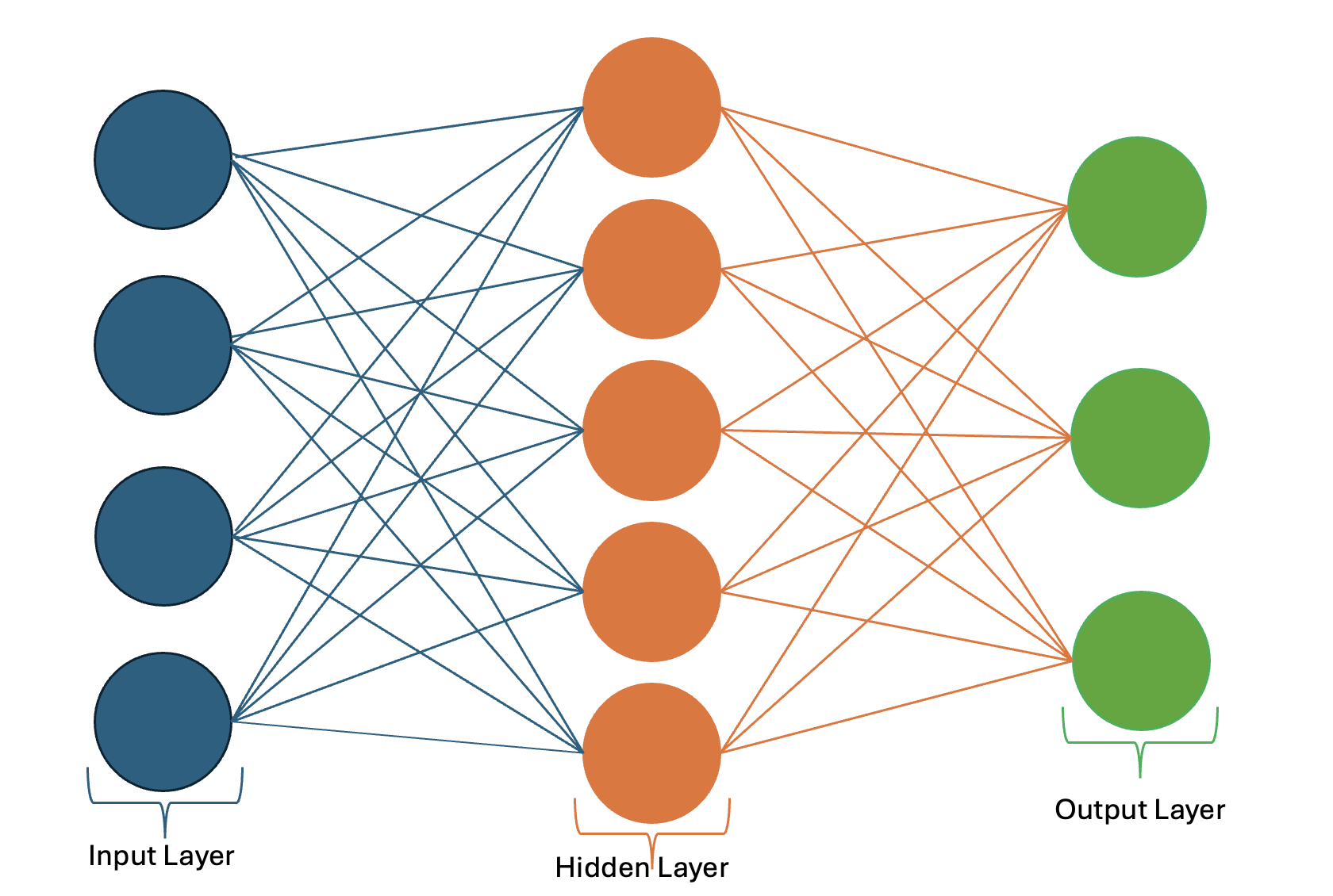
A neural network consists of multiple layers, each performing specific transformations on the input data.

Frequently used Layers in PyTorch:

import torch.nn as nn

fc_layer = nn.Linear(in_features=128, out_features=64)      # Fully Connected Layers

conv_layer = nn.Conv2d(in_channels=3, out_channels=32, kernel_size=3, stride=1, padding=1)  # Convolutional Layers

rnn_layer = nn.RNN(input_size=10, hidden_size=20, num_layers=2, batch_first=True) # Recurrent Layer

dropout_layer = nn.Dropout(p=0.5)

bn_layer = nn.BatchNorm1d(num_features=64)

maxpool_layer = nn.MaxPool2d(kernel_size=2, stride=2)

avgpool_layer = nn.AvgPool2d(kernel_size=2, stride=2)

layer_norm = nn.LayerNorm(normalized_shape=128)

Variations:

• nn.Conv1d, nn.Conv2d, nn.Conv3d
• nn.LSTM → Handles long dependencies.
• nn.GRU → Simpler alternative to LSTM.
• nn.BatchNorm1d, nn.BatchNorm2d, nn.BatchNorm3d
• nn.Dropout1d, nn.Dropout2d, nn.Dropout3d
• nn.MaxPool1d, nn.MaxPool2d, nn.MaxPool3d
• nn.AvgPool1d, nn.AvgPool2d, nn.AvgPool3d
• nn.AdaptiveAvgPool2d → Fixed output size pooling.
• nn.LayerNorm, nn.InstanceNorm2d

Building a Model and Forward Proporgation

There are two ways to define a neural network, the Sequential Class and the Module Class.

Defining a Model with the Sequential Class

The Sequential class is a PyTorch object used to simplify the creation of NN. It allows stacking layers sequentially in the order they are defined without explicitly writing a forward() method. It’s best used for simple models or prototyping.

import torch.nn as nn

model = nn.Sequential(
    nn.Linear(784, 128),  # Input Layer
    nn.ReLU(),            # Activation Layer
    nn.Linear(128, 64),   # Hidden Layer
    nn.ReLU(),            # Activation Function
    nn.Linear(64,10)      # Output Layer
)

Defining a Model with the Module Class

The Module class is the base class for all NN in PyTorch. It provides a framework for defining and organizing the layers of a neural network and enables easy tracking of parameters, gradients, and training. The Forward function defines how the input data is processed through the layers. The .parameters() method (inherited from the Module class) returns the model parameters and is essential for training.

import torch.nn as nn
class SimpleModel(nn.Module):
    def __init__(self):
        super(SimpleModel, self).__init__()
        # Define Layers
        self.fc1 = nn.Linear(in_dim,hidden_dim)
        self.fc2 = nn.Linear(hidden_dim,out_dim)

    def forward(self, x):
        # Define forward pass
        x = self.fc1(x)
        x = nn.ReLU(x)
        x = self.fc2(x)
        return x

Backpropogation

Backpropagation updates the network’s weights based on the gradient of the loss function.

# Define optimizer and loss function
optimizer = torch.optim.Adam(model.parameters(), lr=0.01)
loss_function = nn.MSELoss()

# Example backpropagation
optimizer.zero_grad()  # Clear previous gradients
loss = loss_function(output, torch.tensor([[0.5]]))  # Compute loss
loss.backward()  # Backpropagate
optimizer.step()  # Update weights

Putting it All Together: Training and Testing

We’ve loaded our data into dataloaders

from torch.utils.data import DataLoader, TensorDataset

# Dummy dataset
X_train = torch.rand(100, 10)
y_train = torch.rand(100, 1)
dataset = TensorDataset(X_train, y_train)
dataloader = DataLoader(dataset, batch_size=10, shuffle=True)

We’ve also constructed our model, selected the best loss function and optimizer for our problem, and decided how long to train

import torch.nn as nn
import torch.optim as optim

model = SimpleModel()
loss_fn = nn.MSELoss()
optimizer = optim.Adam(model.parameters(), lr=0.001)  # Pass model.paramters()
epochs = 20

Now we define our training and testing loops.

Training

In PyTorch, we explicitly define how we want to perform training with a training loop. The loop represents one forward and backward pass of one batch.

model.train()
for epoch in range(epochs):                             # loop over epochs
    for x_train, y_train in trainloader:            # loop over batches

        # Send data to GPU (code is the same if no GPU available)
        x_train, y_train = x_train.to(device) , y_train.to(device)

        # Forward Pass
        predicted = model(x_train)

        # Backpropagation - tweak the weights/biases of the NN
        optimizer.zero_grad()                            # Clear previous gradients
        loss = loss_fn(predicted, y_train.reshape(-1,1)) # Compute the loss   
        loss.backward()                                  # Backpropogate
        optimizer.step()                                 # Update weights

Testing

After training, we test the model with unseen data to estimate its general performance. we use torch.no_grad() to tell PyTorch not to compute the gradient. We pass test data through the network once.

model.eval()
num_batch = len(testloader)
loss = 0

with torch.no_grad():
    for x_train, y_train in testloader: # loop over batches

        # send data to GPU (code is the same if no GPU available)
        x_train, y_train = x_train.to(device), y_train.to(device)

        # predict NN output
        predicted = model(x_train)

        # calculate loss
        loss +=loss_fn)predicted,y_train.reshape(-1,1).item()
        # calculate other metrics here
# print result
print('avg loss: {}\t avg accuracy:{}'.format(loss/num_batch, acc/num_batch))

Using a Validation Set

A validation set helps tune hyperparameters and evaluate the model’s generalization ability before final testing. You can use a test loop like the one above to evaluate the validation set after each training epoch.

from sklearn.model_selection import train_test_split

# Splitting data
X_train, X_val, y_train, y_val = train_test_split(X_train, y_train, test_size=0.2, random_state=42)

# Creating DataLoaders
train_dataset = TensorDataset(X_train, y_train)
val_dataset = TensorDataset(X_val, y_val)
train_loader = DataLoader(train_dataset, batch_size=10, shuffle=True)
val_loader = DataLoader(val_dataset, batch_size=10, shuffle=False)